
Mathematical Prerequisites
Overview
This appendix provides the mathematical background necessary to follow the derivations in this book. The Temporal-Momentum Theory (TMT) is formulated using differential geometry, manifold theory, and Lie group theory. Rather than requiring readers to consult external references, we present the essential definitions, theorems, and physical interpretations of these mathematical frameworks as they appear in TMT.
The mathematics is not an arbitrary choice but arises necessarily from the postulate that the metric is null: \(ds_6^{\,2} = 0\). This mathematical structure, properly understood, connects the abstract geometry to physical observables in four dimensions.
—
Differential Geometry
Manifolds and Smooth Structures
A central object in TMT is the compact 2-sphere \(S^2\), which is an example of a smooth manifold. We begin with the precise definitions.
A smooth (or differentiable) manifold of dimension \(n\) is a topological space \(M\) with a smooth structure, meaning:
- \(M\) is a Hausdorff space.
- \(M\) is covered by open sets \(\{U_i\}\), each homeomorphic to an open set in \(\mathbb{R}^n\).
- Transition functions between overlapping charts are smooth (infinitely differentiable).
A smooth map \(f: M \to N\) between manifolds is continuous and smooth in local coordinates. A diffeomorphism is a smooth bijection with smooth inverse.
At each point \(p\) on a smooth manifold \(M\), the tangent space \(T_pM\) is the vector space of all tangent vectors at \(p\). A tangent vector can be represented as a directional derivative acting on smooth functions. The dimension of \(T_pM\) equals the dimension of \(M\). The tangent bundle \(TM\) is the union of all tangent spaces: \(TM = \bigcup_{p \in M} T_pM\).
Given a smooth map \(f: M \to N\) and a point \(p \in M\), the differential (or pushforward) \(df_p: T_pM \to T_{f(p)}N\) is the linear map that takes a tangent vector \(v \in T_pM\) to its image under \(f\). In local coordinates, \(df_p\) is the Jacobian matrix of \(f\) at \(p\).
Vector Fields and Differential Forms
A vector field \(X\) on a manifold \(M\) is a smooth assignment of a tangent vector \(X_p \in T_pM\) to each point \(p \in M\). Vector fields can be added and scaled, forming a module over the ring of smooth functions \(C^\infty(M)\).
A key example is the gradient of a function: if \(f: M \to \mathbb{R}\) is smooth, the gradient vector field \(\nabla f\) points in the direction of steepest increase of \(f\).
A \(k\)-form on a manifold \(M\) is a smooth assignment to each point \(p \in M\) of an alternating multilinear functional on \(T_pM\).
Key examples:
- A 0-form is a smooth function \(f: M \to \mathbb{R}\).
- A 1-form \(\alpha\) assigns to each point and tangent vector a real number: \(\alpha_p: T_pM \to \mathbb{R}\).
- A 2-form \(\omega\) assigns to each point an alternating bilinear functional on pairs of tangent vectors.
- The exterior derivative \(d\) increases the degree by one: \(d: \Omega^k(M) \to \Omega^{k+1}(M)\).
The exterior derivative satisfies \(d^2 = 0\) and is defined without reference to a metric.
The Metric and Connections
A Riemannian metric \(g\) on a smooth manifold \(M\) assigns to each point \(p \in M\) an inner product \(g_p: T_pM \times T_pM \to \mathbb{R}\) that varies smoothly. In local coordinates \((x^1, \ldots, x^n)\), the metric is written:
The metric allows us to measure lengths, angles, and volumes on the manifold. For the 2-sphere \(S^2\) with radius \(R\), the standard metric in spherical coordinates \((\theta, \phi)\) is:
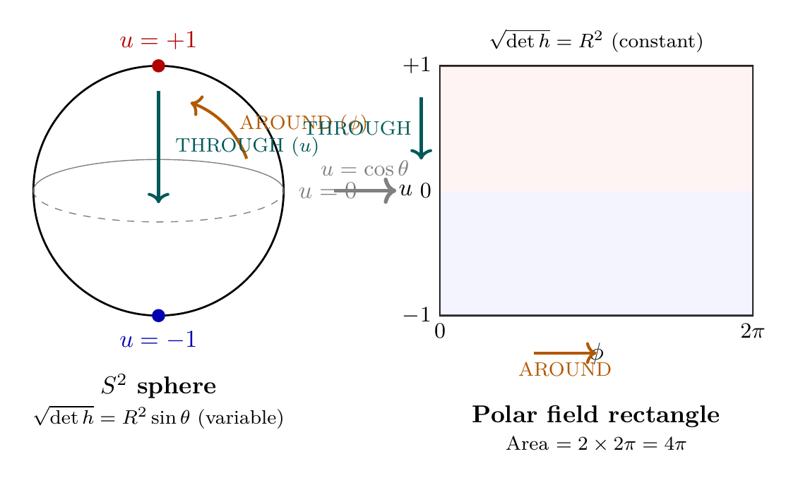
Polar Field Form of the \(S^2\) Metric
The \(S^2\) metric takes a particularly revealing form in the polar field variable \(u = \cos\theta\), where \(u \in [-1, +1]\). Since \(du = -\sin\theta\,d\theta\), we have \(d\theta^2 = du^2/(1-u^2)\) and \(\sin^2\theta = 1-u^2\), giving:
The metric components are \(h_{uu} = R^2/(1-u^2)\) and \(h_{\phi\phi} = R^2(1-u^2)\). Their product gives the key property:
Property | Spherical \((\theta, \phi)\) | Polar \((u, \phi)\) |
|---|---|---|
| Metric components | \(h_{\theta\theta} = R^2\), \(h_{\phi\phi} = R^2\sin^2\theta\) | \(h_{uu} = R^2/(1-u^2)\), \(h_{\phi\phi} = R^2(1-u^2)\) |
| Determinant | \(\det h = R^4\sin^2\theta\) (variable) | \(\det h = R^4\) (constant) |
| Integration measure | \(\sin\theta\,d\theta\,d\phi\) (Jacobian required) | \(du\,d\phi\) (flat Lebesgue) |
| Total area | \(\int_0^\pi\!\sin\theta\,d\theta \int_0^{2\pi}\!d\phi = 4\pi\) | \(\int_{-1}^{+1}\!du \int_0^{2\pi}\!d\phi = 2 \times 2\pi = 4\pi\) |
| Domain shape | \([0,\pi] \times [0,2\pi)\) (variable weight) | \([-1,+1] \times [0,2\pi)\) (flat rectangle) |
Scaffolding note: The polar field variable \(u = \cos\theta\) is a coordinate choice, not a new physical assumption. Both parametrizations describe the same \(S^2\) geometry. The polar form is preferred because the constant metric determinant \(\sqrt{\det h} = R^2\) eliminates the \(\sin\theta\) Jacobian factor from all integrals, making the geometric content of calculations transparent.
An affine connection \(\nabla\) on a manifold \(M\) is a rule for differentiating vector fields. Given vector fields \(X\) and \(Y\), the covariant derivative \(\nabla_X Y\) is another vector field satisfying:
- Linearity: \(\nabla_{aX + bY} Z = a\nabla_X Z + b\nabla_Y Z\) for smooth functions \(a, b\).
- Product rule: \(\nabla_X(fY) = (Xf)Y + f\nabla_X Y\) for smooth \(f\).
- Torsion: The torsion tensor \(T(X,Y) = \nabla_X Y - \nabla_Y X - [X,Y]\) vanishes for a torsion-free connection.
In local coordinates, the connection is specified by Christoffel symbols \(\Gamma^\lambda_{\mu\nu}\):
On a Riemannian manifold, the unique torsion-free connection compatible with the metric is called the Levi-Civita connection. Its Christoffel symbols are given by:
Curvature
The Riemann curvature tensor \(R\) measures how much parallel transport around an infinitesimal loop fails to return a vector to its original value. In components, it is defined through the commutator of covariant derivatives:
For a compact orientable surface \(S\) without boundary:
For the 2-sphere with radius \(R_0\), integration gives:
In the polar field variable \(u = \cos\theta\), the Gauss-Bonnet calculation for \(S^2\) becomes particularly transparent. The Gaussian curvature \(K = 1/R_0^2\) is constant and the area element is the flat measure \(du\,d\phi\), so:
—
Manifold Theory
Classification of Compact 2-Manifolds
A key insight in TMT is that the projection structure between 4D observation and the temporal momentum direction must have the topology of a compact 2-manifold. The following classification theorem determines uniquely which 2-manifold is required.
Every compact connected orientable 2-manifold is diffeomorphic to exactly one of:
- The 2-sphere \(S^2\) (genus 0).
- The 2-torus \(T^2\) (genus 1).
- The connected sum \(\Sigma_g\) of \(g \geq 2\) tori (genus \(g\)).
Two surfaces are diffeomorphic (topologically equivalent in the smooth category) if and only if they have the same genus.
This classification is a classical result from 19th-century differential topology. In TMT, physical constraints (chiral fermions, stability, minimality) force the topology to be \(S^2\) (genus 0).
Euler Characteristic
The Euler characteristic \(\chi(M)\) of a finite CW complex \(M\) is defined as:
Key values:
- \(\chi(S^2) = 2\) (2 vertices, 3 edges, 1 face in one triangulation).
- \(\chi(T^2) = 0\) (flat torus).
- \(\chi(\Sigma_g) = 2 - 2g\) (general surface of genus \(g\)).
For a compact orientable 2-manifold, the integral of the Gaussian curvature equals \(2\pi\) times the Euler characteristic (Gauss-Bonnet theorem, discussed above). This relates a local geometric property (curvature) to a global topological property (Euler characteristic).
Topological vs. Smooth Structure
It is important to distinguish topological and smooth structures.
A homeomorphism is a continuous bijection with continuous inverse. Two topological spaces are homeomorphic if there exists a homeomorphism between them.
A diffeomorphism is a smooth bijection with smooth inverse. Two smooth manifolds are diffeomorphic if there exists a diffeomorphism between them.
Every diffeomorphism is a homeomorphism, but not conversely. Diffeomorphism is a stronger equivalence.
For compact 2-manifolds, every manifold has a smooth structure (in fact, infinitely many). The classification theorem holds in both the topological and smooth categories.
Fiber Bundles
The structure of TMT can be naturally expressed using fiber bundles.
A fiber bundle with total space \(E\), base space \(B\), and fiber \(F\) is a space \(E\) with a surjective map \(\pi: E \to B\) such that:
- For each \(b \in B\), the fiber \(\pi^{-1}(b)\) is homeomorphic to \(F\).
- Locally, \(E\) looks like \(B \times F\): for each \(b \in B\), there exists a neighborhood \(U\) of \(b\) and a homeomorphism \(\phi: \pi^{-1}(U) \to U \times F\) such that \(\pi\) becomes projection onto the first factor.
A principal \(G\)-bundle is a fiber bundle with structure group \(G\) acting on the fibers. The gauge fields of physics are connections on principal bundles.
—
Riemannian Geometry
Geodesics
On a Riemannian manifold, geodesics are the analogs of straight lines.
A curve \(\gamma(t)\) on a Riemannian manifold \((M, g)\) is a geodesic if its acceleration vector is orthogonal to the manifold, i.e., if \(\nabla_{\dot{\gamma}} \dot{\gamma} = 0\). In local coordinates, the geodesic equation is:
Geodesics minimize length locally: a short enough geodesic segment between two points is the shortest curve connecting them.
On \(S^2\), geodesics are great circles (the intersections of the sphere with 2-planes through the center).
Parallel Transport
A vector field \(V\) is parallel along a curve \(\gamma\) if \(\nabla_{\dot{\gamma}} V = 0\). Given an initial vector \(V_0\) at \(\gamma(0)\), parallel transport along \(\gamma\) defines a unique vector field \(V(t)\) satisfying the parallel transport equation.
The parallel transport map \(P_\gamma: T_{\gamma(0)}M \to T_{\gamma(1)}M\) is a linear isomorphism. When the curve is closed, parallel transport around the loop generally does not return vectors to their original position; the failure is measured by the holonomy.
Exponential Map and Logarithmic Coordinates
The exponential map \(\exp_p: T_pM \to M\) at a point \(p\) is defined by:
For a Riemannian manifold, \(\exp_p\) is a diffeomorphism from a neighborhood of the origin in \(T_pM\) to a neighborhood of \(p\) in \(M\) (the normal neighborhood). This allows us to use Cartesian coordinates on \(T_pM\) to describe distances in \(M\).
Curvature and Holonomy
When a vector is parallel transported around a closed loop on a Riemannian manifold, it returns rotated by an angle proportional to the integral of the curvature over the enclosed region. For a simply connected region with small curvature:
On a flat surface (like \(\mathbb{R}^2\)), curvature vanishes and vectors return unchanged. On a curved surface (like \(S^2\)), curvature causes rotation.
In polar field coordinates, the holonomy on \(S^2\) becomes a simple area calculation. For a loop at constant \(u = u_0\) (a latitude circle), the enclosed region is the rectangle \([u_0, +1] \times [0, 2\pi)\) with flat area \((1-u_0) \times 2\pi\). Since \(K = 1/R_0^2\) is constant, the holonomy angle is:
—
Lie Groups and Algebras
Lie Groups and Lie Algebras
Gauge symmetries in physics are described by Lie groups. TMT derives the Standard Model gauge group \(\mathrm{SU}(3) \times \mathrm{SU}(2) \times \mathrm{U}(1)\) from the geometry of \(S^2\).
A Lie group is a smooth manifold \(G\) with a group structure such that:
- Multiplication \(G \times G \to G: (g, h) \mapsto gh\) is smooth.
- Inversion \(G \to G: g \mapsto g^{-1}\) is smooth.
Examples:
- \(\mathbb{R}\) under addition.
- \(\mathbb{R}^+\) under multiplication.
- The circle \(\mathrm{U}(1) = \{z \in \mathbb{C} : |z| = 1\}\) under multiplication.
- The special unitary group \(\mathrm{SU}(n)\): \(n \times n\) unitary matrices with determinant 1.
- The special orthogonal group \(\mathrm{SO}(n)\): \(n \times n\) orthogonal matrices with determinant 1.
The Lie algebra \(\mathfrak{g}\) of a Lie group \(G\) is the tangent space at the identity element \(e\): \(\mathfrak{g} = T_e G\). It is equipped with the Lie bracket \([X, Y] = \lim_{t \to 0} t^{-2}(\exp(tX)\exp(tY)\exp(-tX)\exp(-tY))\) for \(X, Y \in \mathfrak{g}\).
The Lie bracket encodes the local structure of the group. For matrix groups, the Lie bracket is the commutator: \([A, B] = AB - BA\).
Key examples of Lie algebras:
- \(\mathfrak{u}(1)\): the real numbers \(\mathbb{R}\).
- \(\mathfrak{su}(2)\): \(2 \times 2\) traceless skew-Hermitian matrices (dimension 3).
- \(\mathfrak{su}(3)\): \(3 \times 3\) traceless skew-Hermitian matrices (dimension 8).
- \(\mathfrak{so}(3)\): \(3 \times 3\) skew-symmetric real matrices (dimension 3).
The Exponential Map and Representations
For a Lie group \(G\) with Lie algebra \(\mathfrak{g}\), the exponential map \(\exp: \mathfrak{g} \to G\) is defined by:
The exponential map is a local diffeomorphism from a neighborhood of zero in \(\mathfrak{g}\) to a neighborhood of the identity in \(G\).
A representation of a Lie group \(G\) is a smooth homomorphism \(\rho: G \to \mathrm{GL}(V)\), where \(\mathrm{GL}(V)\) is the group of invertible linear transformations of a vector space \(V\).
A representation of the Lie algebra \(\mathfrak{g}\) is a linear map \(\rho: \mathfrak{g} \to \mathfrak{gl}(V)\) (the Lie algebra of \(\mathrm{GL}(V)\)) satisfying \(\rho([X,Y]) = [\rho(X), \rho(Y)]\).
For each Lie group representation, there is an associated Lie algebra representation obtained by differentiating at the identity.
SU(2) and the Isometry Group of \(S^2\)
The isometry group \(\mathrm{Iso}(M)\) of a Riemannian manifold \((M, g)\) is the group of all diffeomorphisms that preserve the metric: \(\phi^* g = g\), where \(\phi^*\) denotes the pullback of the metric.
The isometry group of the round 2-sphere \(S^2\) is:
Every isometry of \(S^2\) extends to an orthogonal transformation of the ambient 3D space.
Polar Field Form of the Killing Vectors
The three Killing vector fields of \(S^2\) take a physically revealing form in polar coordinates \((u, \phi)\). Using \(\partial_\theta = -\sqrt{1-u^2}\,\partial_u\):
The physical content is immediately visible:
- \(K_3 = \partial_\phi\) is a pure AROUND rotation—it moves points horizontally on the polar rectangle \([-1,+1] \times [0,2\pi)\) without changing \(u\). This generates the unbroken \(\mathrm{U}(1)_{\mathrm{em}}\) symmetry.
- \(K_1\) and \(K_2\) mix THROUGH and AROUND—they have both \(\partial_u\) and \(\partial_\phi\) components, coupling the two directions of the polar rectangle. These generate the broken \(W^\pm\) directions.
Killing vector | Spherical \((\theta, \phi)\) | Polar \((u, \phi)\) |
|---|---|---|
| \(K_3\) | \(\partial_\phi\) (pure azimuthal) | \(\partial_\phi\) (pure AROUND) |
| \(K_1, K_2\) | Mix \(\partial_\theta\) and \(\partial_\phi\) | Mix \(\partial_u\) (THROUGH) and \(\partial_\phi\) (AROUND) |
| Physical role | Unbroken vs broken generators | AROUND-only vs mixed directions |
Electroweak symmetry breaking is thus literally the distinction between pure-AROUND and mixed-direction generators on the polar rectangle, a geometric fact that is obscured in the spherical parametrization.
There is a 2-to-1 surjective group homomorphism \(\mathrm{SU}(2) \to \mathrm{SO}(3)\) with kernel \(\pm 1\). Thus, \(\mathrm{SU}(2)\) is the universal cover of \(\mathrm{SO}(3)\):
The Lie algebras are isomorphic: \(\mathfrak{su}(2) \cong \mathfrak{so}(3) \cong \mathbb{R}^3\).
In quantum mechanics, fermions are described by spinor fields, which transform under \(\mathrm{SU}(2)\) (not \(\mathrm{SO}(3)\)). This is because spinors are representations of the double cover, not the original group.
SU(3) from Variable Embedding
The special unitary group \(\mathrm{SU}(n)\) is the group of \(n \times n\) unitary matrices with determinant 1:
The Lie algebra \(\mathfrak{su}(n)\) consists of traceless skew-Hermitian \(n \times n\) matrices. Its dimension is \(n^2 - 1\).
Key dimensions:
- \(\dim \mathfrak{su}(2) = 3\). Generators: Pauli matrices \(\sigma_1, \sigma_2, \sigma_3\) (up to normalization).
- \(\dim \mathfrak{su}(3) = 8\). Generators: Gell-Mann matrices \(\lambda_1, \ldots, \lambda_8\).
In TMT, the \(\mathrm{SU}(3)\) gauge symmetry (color symmetry of the strong force) arises from embedding the projection structure in a way that allows three independent “color” degrees of freedom.
Representations and the Adjoint Action
The adjoint representation of a Lie group \(G\) is the action of \(G\) on its own Lie algebra \(\mathfrak{g}\). For \(g \in G\) and \(X \in \mathfrak{g}\):
The corresponding Lie algebra representation (adjoint representation of \(\mathfrak{g}\)) is:
In gauge theory, the gauge fields transform in the adjoint representation of the gauge group. The Yang-Mills action, central to the Standard Model, is constructed using the adjoint action.
—
Functional Analysis
Hilbert Spaces
The framework for quantum mechanics is Hilbert space. This is the appropriate infinite-dimensional generalization of finite-dimensional vector spaces.
An inner product space is a vector space \(V\) over \(\mathbb{C}\) (or \(\mathbb{R}\)) equipped with an inner product \(\langle \cdot, \cdot \rangle: V \times V \to \mathbb{C}\) satisfying:
- Linearity in the second argument: \(\langle x, ay + bz \rangle = a\langle x, y \rangle + b\langle x, z \rangle\).
- Conjugate symmetry: \(\langle x, y \rangle = \overline{\langle y, x \rangle}\).
- Positive definiteness: \(\langle x, x \rangle \geq 0\), with equality iff \(x = 0\).
The inner product induces a norm \(\|x\| = \sqrt{\langle x, x \rangle}\) and a distance \(d(x,y) = \|x - y\|\).
A Hilbert space is a complete inner product space: an inner product space in which every Cauchy sequence converges. Completeness is essential for analysis, as it ensures that limits of sequences belong to the space.
Examples:
- \(\mathbb{C}^n\) with the standard inner product \(\langle x, y \rangle = \sum_i \bar{x}_i y_i\).
- \(\ell^2(\mathbb{N}) = \left\{(x_1, x_2, \ldots) : \sum_i |x_i|^2 < \infty\right\}\) with \(\langle x, y \rangle = \sum_i \bar{x}_i y_i\).
- \(L^2(\mathbb{R}) = \left\{f: \mathbb{R} \to \mathbb{C} : \int_\mathbb{R} |f(x)|^2\,dx < \infty\right\}\) with \(\langle f, g \rangle = \int_\mathbb{R} \bar{f}(x)g(x)\,dx\).
Linear Operators
A linear operator \(A: H \to H\) on a Hilbert space \(H\) is bounded if there exists \(M > 0\) such that:
The operator norm is defined as:
Examples of bounded operators: matrices (acting on \(\mathbb{C}^n\)), multiplication operators, compact operators.
An unbounded operator \(A\) is defined not on all of \(H\), but on a dense subspace \(\mathrm{Dom}(A) \subset H\) (the domain). Many operators in quantum mechanics are unbounded: the position operator \(\hat{x}\), the momentum operator \(\hat{p}\), and the Hamiltonian \(\hat{H}\) are all unbounded.
For physical observables, we require self-adjoint operators (their own adjoints): \(A = A^\dagger\).
Spectrum and Eigenvalues
For a linear operator \(A\) on a Hilbert space \(H\), the resolvent is:
The spectrum \(\sigma(A)\) is the complement of the resolvent set. For a self-adjoint operator, the spectrum is real.
The spectrum is partitioned into:
- The point spectrum (eigenvalues): values \(\lambda\) such that \(Ax = \lambda x\) for some nonzero \(x\).
- The continuous spectrum: limit points of eigenvalues (not eigenvalues themselves).
- The residual spectrum: part of the spectrum that is neither point nor continuous.
For a self-adjoint operator \(A\) on a Hilbert space \(H\) with spectrum \(\sigma(A)\), there exists a unique spectral measure \(E_\lambda\) such that:
If \(A\) has a discrete spectrum (countable eigenvalues), this becomes:
The spectral theorem justifies diagonalizing hermitian matrices and extends this to infinite-dimensional operators.
Compact Operators
A bounded linear operator \(K: H \to H\) on a Hilbert space is compact if it maps bounded sets to relatively compact sets (closure is compact).
Equivalently, \(K\) is compact if every bounded sequence has a convergent subsequence in the image.
Examples: finite-rank operators, Hilbert-Schmidt operators, integral operators with certain kernels.
If \(K\) is a compact self-adjoint operator on an infinite-dimensional Hilbert space, its spectrum consists of:
- Eigenvalues \(\lambda_n \to 0\) (at most countable).
- Zero (which may or may not be in the spectrum).
- No continuous spectrum.
The eigenvectors form an orthonormal basis for the range of \(K\):
Physical Meaning: Observables and Born Rule
In quantum mechanics, the mathematical framework is interpreted physically as follows:
A quantum observable is a self-adjoint operator \(\hat{A}\) on the Hilbert space of quantum states. Its eigenvalues are the possible measurement outcomes. An eigenstate \(|\psi\rangle\) corresponds to a definite value of the observable.
The spectral theorem ensures that any self-adjoint operator can be written in diagonal form (relative to appropriate basis), making its physical meaning clear.
If a quantum system is in state \(|\psi\rangle\) (normalized: \(\langle \psi |\psi \rangle = 1\)), and we measure an observable \(\hat{A}\) with eigenvalues \(\{a_n\}\) and eigenstates \(\{|n\rangle\}\), then:
- The probability of measuring eigenvalue \(a_n\) is \(P_n = |\langle n |\psi \rangle|^2\).
- After measurement, the state collapses to the eigenstate \(|n\rangle\).
- The expectation value is \(\langle A \rangle = \langle \psi | \hat{A} | \psi \rangle\).
The framework of Hilbert spaces and self-adjoint operators is precisely what is needed for a rigorous mathematical statement of quantum mechanics.
—
Summary and Integration with TMT
This appendix provides the mathematical foundation underlying Temporal-Momentum Theory. The key structures are:
- Differential Geometry: Manifolds, metrics, connections, and curvature form the language for describing curved spacetime and internal symmetries.
- Manifold Theory: The classification of compact 2-manifolds guarantees that the projection structure has topology \(S^2\), derived uniquely from physical constraints.
- Riemannian Geometry: Geodesics, parallel transport, and holonomy connect abstract geometry to the physics of motion and curvature.
- Lie Groups and Algebras: The Standard Model gauge group \(\mathrm{SU}(3) \times \mathrm{SU}(2) \times \mathrm{U}(1)\) is derived from the isometry group of \(S^2\) and its embedding variations.
- Functional Analysis: Hilbert spaces and self-adjoint operators provide the rigorous mathematical framework for quantum mechanics, with the spectral theorem ensuring that observables can be diagonalized.
- Polar Field Coordinates: The variable substitution \(u = \cos\theta\) converts the \(S^2\) metric to a form with constant determinant \(\sqrt{\det h} = R^2\), replacing all trigonometric integrals with polynomial integrals on the flat rectangle \([-1,+1] \times [0,2\pi)\). Killing vectors decompose into pure AROUND (\(K_3 = \partial_\phi\)) and mixed THROUGH/AROUND (\(K_{1,2}\)) directions, making the electroweak symmetry breaking pattern geometric.
These mathematical structures are not imposed externally but emerge from the postulate that the metric is null: \(ds_6^{\,2} = 0\). The mathematics scaffolds the bridge between 4D observation (where we make measurements) and the temporal momentum direction (where time becomes a traversable dimension).
All subsequent chapters of this book rely on the definitions, theorems, and interpretations presented here. The physical predictions of TMT are derived rigorously using these mathematical tools, with every step justified by the theorems and definitions of differential geometry, manifold theory, Lie group theory, and functional analysis.
—
\appendix{Mathematical Prerequisites}
Quick Reference Table:
Concept | Definition/Key Property | Section |
|---|---|---|
| \endhead Smooth Manifold | Hausdorff space with smooth atlas | \Sapp:subsec:manifolds |
| Tangent Space | Vector space of tangent vectors at a point | \Sapp:subsec:manifolds |
| Riemannian Metric | Inner product on tangent spaces, varying smoothly | \Sapp:subsec:metric-connection |
| Christoffel Symbols | Connection coefficients in local coordinates | \Sapp:subsec:metric-connection |
| Riemann Tensor | Curvature measure via commutator of derivatives | \Sapp:subsec:curvature |
| Gaussian Curvature | \(K = R/2\) for 2D surfaces | \Sapp:subsec:curvature |
| Gauss-Bonnet Theorem | \(\int K\,dA = 2\pi\chi(M)\) | Thm thm:app-gauss-bonnet |
| 2-Manifold Classification | Determined by genus \(g\); \(S^2\) has \(g=0\) | \Sapp:subsec:classification-2mflds |
| Euler Characteristic | \(\chi(S^2) = 2\); \(\chi(T^2) = 0\) | \Sapp:subsec:euler-characteristic |
| Lie Group | Smooth manifold with group operations | \Sapp:subsec:lie-defs |
| Lie Algebra | Tangent space at identity with Lie bracket | \Sapp:subsec:lie-defs |
| SO(3) and SU(2) | Isometry of \(S^2\) is SO(3); SU(2) is double cover | Thm thm:app-iso-s2, Thm thm:app-su2-cover-so3 |
| SU(3) | Strong force symmetry; 8 generators | \Sapp:subsec:su3 |
| Hilbert Space | Complete inner product space | \Sapp:subsec:hilbert-spaces |
| Self-Adjoint Operator | Observable in quantum mechanics; spectrum is real | \Sapp:subsec:operators |
| Spectral Theorem | \(A = \int \lambda\,dE_\lambda\) for self-adjoint \(A\) | Thm thm:app-spectral |
| Born Rule | Probability \(P_n = |\langle n|\psi\rangle|^2\) for eigenvalue \(a_n\) | Post post:app-born-rule |
| \multicolumn{3}{l}{Polar Field Coordinate Additions} | ||
| Polar \(S^2\) Metric | \(h_{uu} = R^2/(1-u^2)\), \(h_{\phi\phi} = R^2(1-u^2)\); \(\sqrt{\det h} = R^2\) | \Ssec:appA-polar-s2-metric |
| Flat Integration Measure | \(d\Omega = du\,d\phi\) (constant weight) | Eq. eq:appA-flat-measure |
| Gauss-Bonnet (polar) | \(\int K\,dA = 1 \times 2 \times 2\pi = 4\pi\) (flat rectangle area) | Eq. eq:appA-gauss-bonnet-polar |
| Holonomy (polar) | \(\theta_{\mathrm{hol}} = 2\pi(1-u_0)\) linear in \(u\) | Eq. eq:appA-holonomy-polar |
| Killing Vectors (polar) | \(K_3 = \partial_\phi\) pure AROUND; \(K_{1,2}\) mix THROUGH/AROUND | \Ssec:appA-polar-killing |