The Temporal Persistence of S²
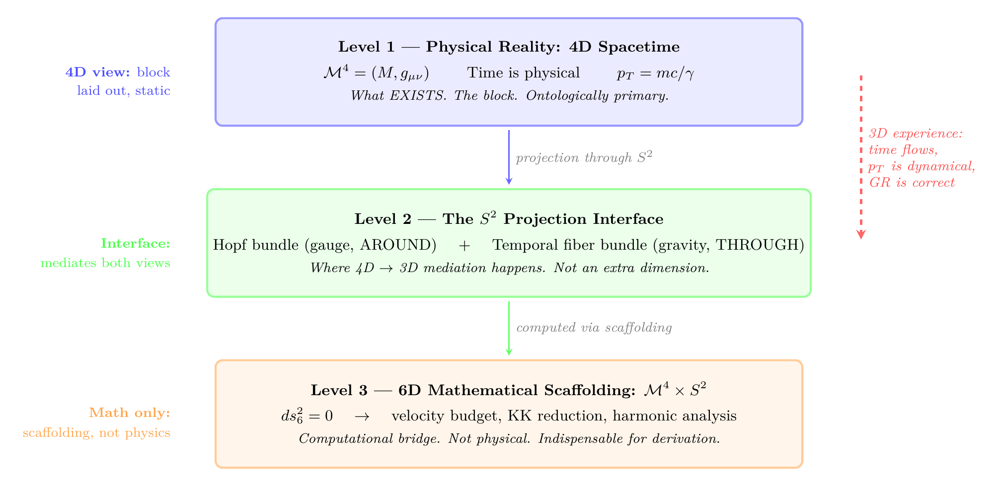
Scaffolding interpretation. We live in a 4D world. Time is not merely a coordinate — it is a physical dimension where temporal momentum lives. What we observe as matter in three spatial dimensions IS temporal momentum on the \(S^2\) projection structure.
The \(\mathcal{M}^4 \times S^2\) product metric is mathematical scaffolding — the 6D framework where the full structure converges, not a claim about physical hidden dimensions. The scaffolding lets us compute how the \(S^2\) interface mediates the 4D \(\to\) 3D projection; the interface itself is physical. Gravity and time emerge from the vertical (THROUGH) component of the Hopf bundle on \(S^2\).
This chapter requires both perspectives:
- 4D (the block): Spacetime is laid out, complete. \(S^2\) is at every event. The modulus field \(\sigma(x)\) is a configuration on the block. Nothing “flows.”
- 3D (the experience): We are temporal momentum beings, progressing through time at speed \(v_T = c/\gamma\). Gravity affects our progression. Persistence is the continuity of physics from one moment to the next.
Both describe the same reality. The 6D scaffolding is the mathematical bridge between them.
The Two Perspectives
Before any theorem, before any equation, we must establish the conceptual framework that governs everything in this chapter — and, indeed, everything in TMT.
There are two equally valid ways to describe the same physical reality. Neither is wrong. Neither is approximate. They are the same geometric truth seen from different sides of the \(S^2\) interface.
The physics of temporal persistence admits two complete, self-consistent descriptions:
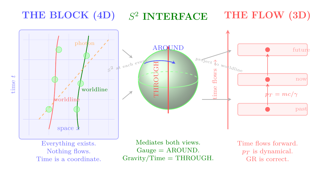
- (I) The 4D Perspective (The Block). Spacetime \(\mathcal{M}^4\) exists as a complete, static, four-dimensional manifold. Every event — past, present, future — is equally real, equally present. Time is a coordinate, not a process. The \(S^2\) interface is at every event \(x \in \mathcal{M}^4\). The modulus field \(\sigma(x)\) is a scalar field configuration on the block — it does not “evolve,” it simply has a shape. Worldlines are geometric curves embedded in the block. They do not “travel” from one event to another any more than a line drawn on paper travels from one end to the other. The block merely IS — now, forever, all that is and was, laid out.
- (II) The 3D Perspective (The Experience). We are three-dimensional beings. We observe three spatial dimensions. We experience time as a forward progression — one moment after another, irreversibly, carrying us from past through present toward future. This experience is not an illusion. It is the correct description of what it is like to be an entity whose worldline winds through the \(S^2\) fiber structure within the 4D block.
Gravity, from this perspective, is the geometric configuration of the \(S^2\) fiber across the block. Where \(\sigma(x)\) varies (near masses), the fiber radius changes from event to event. This variation IS gravity. It is not a force acting on the block; it is a property of the block's geometry. The Einstein equations \(G_{\mu\nu} = 8\pi G_4 T_{\mu\nu}\) are constraints on which block configurations are self-consistent, not dynamical equations describing evolution.
From this perspective, temporal momentum \(p_T = mc/\gamma\) is real, dynamical momentum. It measures how fast we progress through the block. The velocity budget \(v^2 + v_T^2 = c^2\) is a dynamical law: move faster through space, and you move slower through time. General relativity is correct — time dilation, gravitational redshift, the twin paradox — all of it happens, experienced by 3D entities whose temporal momentum varies with velocity and gravitational potential. Gravity is a real force that affects our temporal progression. The modulus wave equation \(\Box\sigma = \rho_{p_T} c/(2M_{\text{Pl}})\) is a real dynamical equation propagating the interface geometry forward in time. The persistence of \(S^2\) from one moment to the next is what makes physics continuous — it is why there IS a next moment.
The two perspectives are related by the \(S^2\) projection interface:
The 4D perspective is ontologically primary: it describes what EXISTS. The 3D perspective is experientially primary: it describes what we OBSERVE. The 5D and 6D mathematical scaffolding is the computational bridge: it provides the tools (\(ds_6^2 = 0\), harmonic analysis, KK reduction) for deriving one from the other.
As a FRAMEWORK principle, the Dual Perspective Principle is not provable in the mathematical sense — it is an interpretive commitment governing how the mathematics maps to physical reality. We justify each component:
(I): The 4D block perspective is the content of general relativity's geometric formulation. The spacetime manifold \((\mathcal{M}^4, g_{\mu\nu})\) is defined as a complete, connected, 4-dimensional pseudo-Riemannian manifold. Points on the manifold are events; they exist independently of any observer or any foliation into spatial slices. The Einstein equations are tensor equations on \(\mathcal{M}^4\) — they constrain the relationship between geometry and matter content at every event simultaneously, not sequentially. TMT enriches this by attaching an \(S^2\) fiber at every event, but the block character is standard GR.
(II): The 3D experiential perspective follows from the null constraint \(ds_6^2 = 0\) (P1). An entity with winding number \(n \neq 0\) (massive) has its worldline constrained by:
(Equivalence): The two descriptions are related by projection. The 4D block contains all worldlines. Restricting to a single worldline and parameterising by proper time \(\tau\) recovers the 3D experiential description. Conversely, assembling all possible worldlines and their mutual relationships (via the Einstein equations) reconstructs the block. The \(S^2\) interface mediates this projection: it is the geometric structure at each event that determines how the 4D block decomposes into 3D spatial slices plus temporal progression.
A common error in physics is to privilege one perspective and dismiss the other. The “block universe” camp says time is an illusion. The “presentist” camp says only the present is real. TMT does not take sides. Both perspectives are complete descriptions of the same geometric reality, related by the \(S^2\) projection.
The 4D perspective is needed for: global questions (topology of spacetime, conservation of \(c_1\), existence and uniqueness of solutions), the scaffolding doctrine (keeping 6D as mathematics, not physics), and understanding why the universe “merely is.”
The 3D perspective is needed for: all of experimental physics (we ARE 3D observers), dynamical questions (how does a clock tick? what does an accelerating observer experience?), and understanding temporal momentum as a real, measurable quantity (\(p_T = mc/\gamma\) has units, can be measured, and obeys conservation laws).
The scaffolding (5D/6D) is needed for: computing the relationship between the two. The velocity budget \(v^2 + v_T^2 = c^2\) is derived from \(ds_6^2 = 0\) (scaffolding), but it IS the bridge between the 4D constraint (worldlines are null in 6D) and the 3D experience (time slows when you move).
Temporal momentum is the movement of 3D space across time.
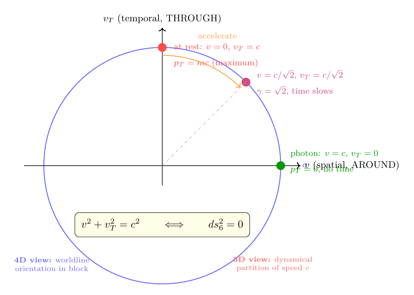
This is not a metaphor. The velocity budget \(v^2 + v_T^2 = c^2\) partitions every entity's total speed \(c\) into spatial velocity \(v\) (movement through 3D) and temporal velocity \(v_T\) (movement through time). Temporal momentum \(p_T = mv_T = mc/\gamma\) is the momentum associated with this temporal motion.
From 3D: Temporal momentum is what makes you a temporal being. A particle at rest (\(v = 0\)) has \(v_T = c\) — it moves through time at the speed of light. Its rest energy \(E_0 = mc^2\) IS the kinetic energy of this temporal motion. Mass is not a static label; it is the dynamical consequence of moving through time. When you accelerate (\(v\) increases), \(v_T\) decreases — you move more slowly through time. This IS time dilation. When you enter a gravitational well, the modulus \(\sigma\) changes the local fiber geometry, altering \(v_T\) — this IS gravitational time dilation. General relativity is correct because it correctly describes the dynamics of temporal progression.
From 4D: Temporal momentum is a geometric property of worldline orientation within the block. A massive worldline (winding number \(n \neq 0\)) has a nonzero projection onto the THROUGH direction at every event. The magnitude of this projection is \(p_T\). The worldline is “tilted” relative to the \(S^2\) fiber structure — more spatial velocity means more tilt away from the fiber axis, less temporal projection, less \(p_T\). But nothing “moves” — the worldline simply has this orientation, laid out in the block.
Both descriptions are the same worldline viewed from different levels of the ontological architecture. The \(S^2\) interface is where they meet.
The Problem: \(S^2\) Must Persist
Chapter 157 established the topological structure of \(S^2\): the Hopf fibration \(S^1 \hookrightarrow S^3 \to S^2\), the vertical/horizontal decomposition \(T_pS^3 = V_p \oplus H_p\), and the conservation laws mandated by bundle non-triviality (\(c_1 = 1\)). But every result in Chapter 157 describes \(S^2\) at a single event. The Hopf bundle is a spatial object — a principal \(\text{U}(1)\)-bundle over \(S^2\) at a fixed spacetime point. The velocity budget \(v^2 + v_T^2 = c^2\) allocates motion between spatial (AROUND) and temporal (THROUGH), but does not explain how the interface at one event connects to the interface at another.
From the two perspectives, this problem takes different forms:
- (I) 4D formulation (the block): Given that \(S^2\) is the projection interface at each event, what constrains the configuration of the \(S^2\) fiber across the spacetime manifold \(\mathcal{M}^4\)? What geometric conditions ensure that the fiber at event \(x\) is related to the fiber at event \(x'\) in a way that preserves all topological invariants and is self-consistent with the Einstein equations?
- (II) 3D formulation (the experience): Given the \(S^2\) interface at time \(t\) with its Hopf bundle structure, gauge connection, and monopole topology, what determines \(S^2\) at time \(t + dt\)? What is the mechanism that propagates the interface forward along our worldline?
Answer: The modulus field \(\sigma(x) = R(x)/R_0 - 1\) is a scalar field on \(\mathcal{M}^4\) whose configuration is constrained by the tracelessness condition \(T^A_A = 0\). This constraint, together with the topological invariance of \(c_1 = 1\), determines the complete fiber geometry across the block. The block configuration is unique (given boundary conditions) and self-consistent.
Answer: The modulus wave equation \(\Box\sigma = \rho_{p_T} c/(2M_{\text{Pl}})\) is a hyperbolic PDE that propagates initial data forward in time. Given \(\sigma\) and \(\dot\sigma\) on a Cauchy surface, the future (and past) of the fiber geometry is uniquely determined. Gravity — through the modulus field — is the mechanism.
These are the same answer expressed in different languages. The 4D constraint on the block configuration IS the 3D wave equation viewed from the block perspective. The 3D wave equation IS the 4D constraint restricted to a foliation.
(I): The product metric (Lemma lem:ch157-decoupling) generalises to:
(II): The tracelessness condition, when decomposed as \(T^\mu_\mu + T^i_i = 0\) and the \(S^2\) contributions are evaluated, gives the modulus wave equation (derived in \Ssec:ch158-modulus-derivation). This is a hyperbolic PDE with well-posed initial value problem (Hawking & Ellis 1973, Theorem 7.4.3).
(Equivalence): A Lorentzian manifold is globally hyperbolic if and only if it admits a Cauchy surface. The block (maximal development) is the union of all Cauchy developments. The wave equation on the block is the statement that the constraint equations hold everywhere. Restricting to a foliation \(\Sigma_t\) recovers the initial-value formulation. □ □
The Central Claim
We can now state the central claim of this chapter in language that respects both perspectives:
Temporal momentum is the movement of 3D space across time.
From 3D: We are entities embedded in a 4D block, experiencing time as forward progression because our worldlines wind through the \(S^2\) fiber structure. Temporal momentum \(p_T = mc/\gamma\) measures the rate of this progression. Mass is the compaction of temporal momentum into a 3D observable. Rest energy \(E_0 = mc^2\) is the kinetic energy of temporal motion.
From 4D: The block is laid out, complete, static. Worldlines are geometric curves. Mass is the winding number of the worldline around the \(S^1\) fiber. Gravity is the variation of the \(S^2\) fiber geometry across the block. Time does not flow — it is a coordinate, one of four.
The \(S^2\) interface relates both views: it is the geometric structure at each event that determines how 4D existence projects to 3D experience. Get the \(S^2\) structure right — get gravity and time right — and the universe unfolds.
TMT at its core is about gravity and time. The gauge forces (AROUND, horizontal) are topology. Gravity and time (THROUGH, vertical) are geometry. P1 (\(ds_6^2 = 0\)) is the single equation that generates both, through the velocity budget and the \(S^2\) projection. Every result across 150+ chapters — every coupling constant, every mass hierarchy, every conservation law — traces back to the correct treatment of temporal momentum on the \(S^2\) interface.
The Spacetime Fiber Bundle
Chapter 157 constructed a fiber bundle over \(S^2\): the Hopf bundle \(S^1 \hookrightarrow S^3 \to S^2\) encoding gauge structure. We now construct a second fiber bundle — over four-dimensional spacetime — encoding gravitational structure.
The spacetime fiber bundle is:
- The base space is the 4D spacetime \(\mathcal{M}^4\) with Lorentzian metric \(g_{\mu\nu}\).
- The fiber over each spacetime event \(x\) is \(S^2(x)\), the interface at \(x\), equipped with its round metric of radius \(R(x)\), its Hopf bundle structure, and its monopole.
- The projection \(\pi\) maps each point of \(S^2(x)\) to its spacetime label \(x\).
- The structure group is \(\text{CO}^+(2) = \mathbb{R}_+ \times \text{SO}(3)\), the group of orientation-preserving conformal transformations of \(S^2\). A change of fiber from \(S^2(x)\) to \(S^2(x + dx)\) decomposes into:
- A conformal rescaling by \(R(x + dx)/R(x) = 1 + \partial_\mu\sigma\,dx^\mu\), parameterised by the modulus gradient \(\partial_\mu \sigma\).
- An \(\text{SO}(3)\) rotation, parameterised by a rotation matrix \(\Lambda^i{}_j(x, dx)\) relating the frame on \(S^2(x)\) to the frame on \(S^2(x + dx)\).
The full structure group \(\text{CO}^+(2) = \mathbb{R}_+ \times \text{SO}(3)\) allows both conformal rescaling and rotation of the \(S^2\) fiber. For the product metric ansatz used throughout this chapter, the \(\text{SO}(3)\) component is trivially realised: the mixed Christoffel symbols are pure scaling (\(\Gamma^i_{\mu j} \propto \delta^i_j\), Eq. eq:ch158-mixed-christoffel), so \(\omega_\text{rot} = 0\) (Eq. eq:ch158-rotation-flat). The effective structure group reduces to \(\mathbb{R}_+\) (conformal rescaling only).
The full \(\text{SO}(3)\) becomes physically relevant when the product structure is broken: frame-dragging near a Kerr black hole introduces gravitomagnetic \(\text{SO}(3)\) rotations of the fiber frame, and the Berry phase of parallel-transported fibers around closed spacetime loops can be nontrivial. These effects are treated in the chapters on rotating spacetimes.
Given the product metric ansatz \(g_{AB}\,dx^A dx^B = g_{\mu\nu}(x)\,dx^\mu dx^\nu + R^2(x)\,\hat{g}_{ij}(y)\,dy^i dy^j\) with \(S^2\) fibers carrying their round metric, the fiber bundle \(\mathcal{E} \to \mathcal{M}^4\) with structure group \(\text{CO}^+(2)\) is unique up to bundle isomorphism.
The fiber is \(S^2\) with its round metric of variable radius \(R(x)\). The transition functions between coordinate patches on \(\mathcal{M}^4\) must preserve the round metric up to a conformal factor (rescaling by \(R(x')/R(x)\)) and an isometry (\(\text{SO}(3)\) rotation). These are precisely the elements of \(\text{CO}^+(2)\). A bundle with fibers \((S^2, R^2 \hat{g})\) and a different structure group \(G \neq \text{CO}^+(2)\) would either fail to preserve the round metric (if \(G\) is too large) or fail to allow radius variation (if \(G\) does not contain \(\mathbb{R}_+\)). Isomorphism classes of principal \(\text{CO}^+(2)\)-bundles over \(\mathcal{M}^4\) are classified by \(H^1(\mathcal{M}^4; \text{CO}^+(2))\). Since \(\text{CO}^+(2)\) is connected and \(\mathcal{M}^4\) is simply connected (for cosmologically relevant spacetimes), this cohomology is trivial, giving a unique bundle. □ □
The modulus field \(\sigma(x, t)\) depends on all four spacetime coordinates, not just time. Near a massive object, \(\sigma = -GM/(rc^2)\) varies spatially. A gravitational wave has \(\sigma \sim h(t - x/c)\), varying in both space and time. A bundle over \(\mathbb{R}\) (time alone) would collapse all spatial dependence and lose the gravitational field content. The curvature of the spacetime fiber bundle is a 2-form on \(\mathcal{M}^4\); since \(\mathcal{M}^4\) is four-dimensional, non-trivial 2-forms exist. (On \(\mathbb{R}\), all 2-forms vanish identically.)
Perspective note: From 4D (the block), \(\mathcal{M}^4\) is the natural base because the block IS \(\mathcal{M}^4\) — the fiber varies over the entire manifold, not just along one direction. From 3D (the experience), restricting the bundle to a single worldline \(\gamma: \mathbb{R} \to \mathcal{M}^4\) gives a bundle over \(\mathbb{R}\) — the “temporal fiber bundle” of the Core Principles — which describes the fiber sequence that one observer experiences. Both are valid: \(\mathcal{E} \to \mathcal{M}^4\) is the global structure; \(\gamma^*\mathcal{E} \to \mathbb{R}\) is the experiential restriction.
Connection Decomposition
The connection on \(\mathcal{E} \to \mathcal{M}^4\) decomposes according to the Lie algebra splitting \(\mathfrak{co}^+(2) = \mathbb{R} \oplus \mathfrak{so}(3)\):
The spacetime fiber bundle \(\mathcal{E} \to \mathcal{M}^4\) carries a connection determined by P1, with two components:
- (a) The conformal (scalar) connection \(\omega_{\text{conf}}\), an \(\mathbb{R}\)-valued 1-form on \(\mathcal{M}^4\):
- (b) The rotational (SO(3)) connection \(\omega_{\text{rot}}\), an \(\mathfrak{so}(3)\)-valued 1-form on \(\mathcal{M}^4\):
- (c) Flat connection (\(\partial_\mu\sigma = 0\), \(\omega_\text{rot} = 0\)): the interface does not change from point to point. From 4D: the block has uniform fiber geometry everywhere. From 3D: no gravity, no time variation, Minkowski spacetime.
- (d) Curved connection (\(\partial_\mu\sigma \neq 0\) near a mass):
From 4D: \(\omega_\text{conf}\) is a 1-form on the block — a geometric object that exists at every event, encoding how the fiber radius varies across the manifold.
From 3D: Along a worldline, \(\omega_\text{conf}(\dot\gamma) = \dot\sigma/(1+\sigma)\) measures how fast the fiber radius is changing as the observer progresses through time. Near a mass: \(\omega_\text{conf}(\partial_r) = GM/(r^2 c^2)\) — the gravitational field.
(a): The conformal connection measures \(d\ln R\). Since \(R(x) = R_0(1 + \sigma(x))\), we have \(d\ln R = d\sigma/(1+\sigma)\). This is a standard result: for a fiber bundle whose fiber is parameterised by a single scale factor, the connection on the \(\mathbb{R}_+\) component is \(d\ln(\text{scale})\).
(b): The mixed Christoffel symbols for a product metric \(g = g^{(1)}_{\mu\nu}(x)\,dx^\mu dx^\nu + R^2(x)\hat{g}_{ij}(y)\,dy^i dy^j\) are:
(c): \(\partial_\mu \sigma = 0 \Rightarrow R(x) = R_0 \Rightarrow\) the fiber is constant across spacetime.
(d): Near a static, spherically symmetric mass \(M\), the tracelessness condition gives \(\nabla^2 \sigma = \rho_{p_T} c/(2M_{\text{Pl}})\). The Green's function solution is \(\sigma = -GM/(rc^2)\). □ □
The Curvature of the Spacetime Fiber Bundle
The curvature of the conformal connection \(\omega_\text{conf} = \partial_\mu \sigma\,dx^\mu\) is:
The physical gravitational curvature enters through the spacetime metric. The modulus field sources spacetime curvature via the Einstein equations:
From 4D: The Riemann tensor \(R^\alpha{}_{\beta\mu\nu}\) is a property of the block geometry — it exists at every event. It is non-zero wherever \(\sigma\) has non-trivial gradients.
From 3D: The Riemann tensor produces tidal forces, geodesic deviation, and the observable effects of gravity. These are what 3D entities experience as “gravitational attraction.”
Both are the same tensor. One description says “the block has this curvature.” The other says “we feel this force.”
The vanishing of \(\Omega_\text{conf}\) follows from \(d^2 = 0\) applied to \(\omega_\text{conf} = d\sigma\). For the Einstein equations: the 6D Einstein tensor decomposes (Chapter 52) into \(G^{(4)}_{\mu\nu}\), modulus terms, and \(S^2\) sector. The 4D coupling \(G_4\) is related to the 6D coupling by \(M_{\text{Pl}}^2 = 4\pi R_0^2 M_*^4\). □ □
The vanishing of \(\Omega_\text{conf}\) may appear to contradict the existence of gravity, but these are different kinds of curvature. The conformal connection is abelian (\(\mathbb{R}\)-valued), and every abelian connection on a contractible base is flat — this is a mathematical triviality (\(d^2 = 0\)), not a physical statement.
Gravitational content enters not through the fiber bundle curvature \(\Omega_\text{conf}\), but through the spacetime curvature \(R^\alpha{}_{\beta\mu\nu}\), which depends on second derivatives of the modulus field \(\sigma\) (through the Einstein equations). The fiber bundle formalism captures the first-order structure (how \(\sigma\) varies from point to point); gravity lives in the second-order structure (how that variation itself varies — i.e., tidal effects).
Concretely: the Newtonian potential \(\sigma = -GM/(rc^2)\) has \(\partial_\mu\sigma \neq 0\) (gravitational field) and \(\partial_\mu\partial_\nu\sigma \neq 0\) (tidal field), but the abelian curvature \(\Omega = d(d\sigma) = 0\) vanishes identically. The physics is in \(R^\alpha{}_{\beta\mu\nu}\), not in \(\Omega_\text{conf}\).
| Hopf Bundle (Ch 157) | Spacetime Bundle (This Chapter) | |
|---|---|---|
| Base | \(S^2\) | Spacetime \(\mathcal{M}^4\) |
| Fiber | \(S^1\) (temporal orbit) | \(S^2(x)\) (interface at event \(x\)) |
| Total space | \(S^3 \cong \text{SU}(2)\) | \(\mathcal{E} = \bigsqcup_x S^2(x)\) |
| Structure group | \(\text{U}(1)\) | \(\text{CO}^+(2) = \mathbb{R}_+ \times \text{SO}(3)\) |
| Connection | Hopf connection \(\mathcal{A}\) | \(\omega_\text{conf} = \partial_\mu\sigma\,dx^\mu\) |
| Curvature | \(F = \frac{1}{2}\omega_{S^2}\) (gauge field) | \(R^\alpha{}_{\beta\mu\nu}\) (spacetime) |
| Physical content | Gauge forces (AROUND) | Gravity and time (THROUGH) |
| Perspective | Topology at a single event | Geometry across the block |
| Non-triviality | \(c_1 = 1\) (monopole) | \(\partial_\mu\sigma \neq 0\) (mass present) |
The \(S^2\) interface is the meeting point. Gauge forces live ON \(S^2\) (Hopf bundle, AROUND). Gravity IS the variation of \(S^2\) across spacetime (spacetime bundle, THROUGH). These are orthogonal directions in the Hopf decomposition \(T_pS^3 = V_p \oplus H_p\) — maximally separated within a unified structure. This is why gauge forces and gravity look so different phenomenologically: they ARE different directions. But they emerge from the same geometric object (\(S^2\)) through the same postulate (P1).
The Modulus Wave Equation: From Tracelessness to Dynamics
The modulus wave equation is the dynamical heart of temporal persistence. This section derives it from the tracelessness condition, providing dimensional analysis and factor origins.
The modulus field \(\sigma(x) = R(x)/R_0 - 1\) satisfies:
From 4D: This is a constraint on the block. It determines which configurations \(\sigma(x)\) on \(\mathcal{M}^4\) are self-consistent with the matter content \(\rho_{p_T}(x)\). The operator \(\Box\) is defined on the full manifold simultaneously, not sequentially.
From 3D: This is a wave equation. Given initial data \((\sigma, \dot\sigma)\) on a spacelike surface, it propagates the interface geometry forward in time. The source \(\rho_{p_T} c/(2M_{\text{Pl}})\) says: temporal momentum sources tell the interface how to curve.
Step 1 (Dimensional check): \(\sigma\) is dimensionless. \(\Box\sigma\) has dimensions \([\text{length}]^{-2}\). The right-hand side: \([\rho_{p_T} c / M_{\text{Pl}}] = [\text{kg}\,\text{m}^{-2}\,\text{s}^{-1}] \cdot [\text{m}\,\text{s}^{-1}] / [\text{kg}] = [\text{m}^{-2}]\). \(\checkmark\)
Step 2 (The tracelessness condition): On the \(\mathcal{M}^4 \times S^2\) scaffolding, the total 6D stress-energy satisfies \(T^A_A = 0\) (the null constraint \(ds_6^2 = 0\) implies the total energy-momentum trace vanishes; Chapter 52, \S52.2). Decomposing into 4D and \(S^2\) sectors:
Step 3 (The \(S^2\) trace): The \(S^2\) fiber metric is \(g_{ij}(x) = R^2(x)\,\hat{g}_{ij}\) where \(R(x) = R_0(1+\sigma(x))\). The \(S^2\) contribution to the Ricci tensor gives (Chapter 52, \S52.3):
Step 4 (The 4D trace): For non-relativistic matter, \(T^\mu_\mu = -\rho c^2 = -\rho_{p_T}\,c\), where \(\rho_{p_T} = \rho_0 c\) is the temporal momentum density (the matter content couples through temporal momentum, not through bare energy; P3).
Step 5 (Assembly): Substituting Steps 3 and 4 into the tracelessness condition \(T^\mu_\mu + T^i_i = 0\):
Step 6 (The modulus wave equation): Rearranging Step 5 and absorbing the potential into the wave operator (in the linearised regime where \(|\sigma| \ll 1\) and \(V'(\sigma)/M_{\text{Pl}}^2 \ll \Box\sigma\), which holds away from the Planck scale):
Factor | Value | Origin | Source |
|---|---|---|---|
| \(\Box\) | d'Alembertian | Wave operator on \(\mathcal{M}^4\) | Standard GR |
| \(\sigma\) | \(R/R_0 - 1\) | Modulus perturbation | Def. (this chapter) |
| \(2\) in denominator | \(1/2\) | Two \(S^2\) dimensions in \(T^i_i\) | \(T^A_A = 0\) decomposition |
| \(M_{\text{Pl}}\) | \(\sqrt{\hbar c/(8\pi G)}\) | Scaffolding volume relation \(M_{\text{Pl}}^2 = 4\pi R_0^2 M_*^4\) | Ch 52, \S52.3 |
| \(\rho_{p_T}\) | \(\rho_0 c\) | Temporal momentum density (P3) | Ch 52 |
| \(c\) | speed of light | From \(T^\mu_\mu = -\rho_{p_T} c\) | Ch 52 |
In vacuum (\(\rho_{p_T} = 0\)): \(\Box\sigma = 0\). From 4D: the unique static, spherically symmetric block configuration with \(\sigma \to 0\) at infinity is \(\sigma = 0\) (flat space). From 3D: the interface is uniform, no gravity, no time variation. Near a point mass: \(\sigma = -GM/(rc^2)\), reproducing the Newtonian potential.
Polar Coordinate Form
In polar field coordinates \(u = \cos\theta\) on \(S^2\) (where \(\theta\) is the polar angle from the temporal axis), the velocity budget and modulus equation take dual forms:
The velocity budget \(v^2 + v_T^2 = c^2\) becomes \(c^2(1-u^2) + c^2 u^2 = c^2\), manifestly an identity for all \(u \in [-1, 1]\). The two poles \(u = \pm 1\) correspond to purely temporal motion (\(v = 0\), particle at rest); the equator \(u = 0\) corresponds to purely spatial motion (\(v_T = 0\), photon).
The modulus wave equation in polar coordinates on a spherically symmetric background \(\sigma = \sigma(r)\) becomes:
Dual Spheres: The Temporal Pair
For two spacetime events \(x\) and \(x' = x + \Delta x\) with \(\Delta x\) finite, the dual sphere pair is:
From 4D: The dual pair is a geometric relationship between two fibers in the block. Both fibers exist; the parallel transport map compares them.
From 3D: The dual pair is what an observer experiences over a finite time interval: the interface “now” (\(S^2(x)\)) and the interface “then” (\(S^2(x')\)). The parallel transport is gravity connecting the two moments.
Physics as the Temporal Sequence of Dual Pairs
What we observe as physics is the temporally ordered sequence of \(S^2\) fibers along a worldline:
Each physical phenomenon maps to a property of this sequence:
- (a) Time = the parameter \(\tau\) labeling the sequence. From 3D: “the passage of time” — one moment after the next. From 4D: \(\tau\) is the arc-length along a timelike curve in the block.
- (b) Mass = the temporal momentum \(p_T = mc/\gamma\). From 3D: the rate at which a particle traverses the temporal orbit (\(S^1\) fiber within each \(S^2\)). Mass is not static — it is the dynamical consequence of temporal motion. \(m = n\hbar/(R_0 c)\) from the integer winding number \(n\). From 4D: \(n\) is a topological property of the worldline's winding in the fiber — it just IS that integer, laid out in the block.
- (c) Gravity = the parallel transport map \(\Phi\). From 3D: when \(\Phi\) is non-trivial, the fiber geometry changes from one event to the next, and freely falling particles follow geodesics. From 4D: \(\Phi\) encodes how the fiber geometry varies across the block. Gravity IS the interface (Core Principles \S9) — not a force ON \(S^2\) but a property of \(S^2\)'s variation across \(\mathcal{M}^4\).
- (d) Gravitational time dilation = the conformal factor \(R(x')/R(x)\). From 3D: clocks tick slowly near masses because the fiber geometry changes the local temporal velocity. \(d\tau/dt = \sqrt{1 + 2\sigma}\). From 4D: the block simply has a different fiber radius at different events. No “slowing” — just geometry.
- (e) Gauge forces = the internal structure of each \(S^2(x)\). These are AROUND quantities: \(g^2 = 4/(3\pi)\) is an overlap integral on a single \(S^2\), independent of the spacetime sequence. The gauge coupling does not vary with \(\sigma\) — it is topological.
(a): By construction, the worldline is parameterised by proper time \(\tau\). The spacetime fiber bundle assigns an \(S^2\) at each event.
(b): From the velocity budget, \(v_T = c\cos\theta\). Mass \(m = n\hbar/(R_0 c)\) from the winding number. The \(S^1\) fiber has circumference \(2\pi R_0\).
(c): The parallel transport \(\Phi\) is determined by the connection (Theorem thm:ch158-grav-connection). When \(\partial_\mu\sigma = 0\), \(\Phi = \text{id}\) and spacetime is flat. When \(\partial_\mu\sigma \neq 0\), the fiber geometry changes along the worldline.
(d): \(d\tau^2 = (1 - r_s/r)\,c^2 dt^2 - \ldots = (1 + 2\sigma)\,c^2 dt^2 - \ldots\)
(e): \(g^2 = 4/(3\pi)\) is computed from monopole harmonic overlaps on a single \(S^2\) — a topological/geometric invariant independent of \(\sigma\). □ □
The \(S^2\) Is Not Static
The \(S^2\) interface has time-dependent and time-independent quantities, and the distinction is sharp:
What changes (from event to event across the block; experienced as dynamics in 3D):
- (a) The radius \(R(x) = R_0(1 + \sigma(x))\). Perturbations \(\sigma(x)\) propagate as gravity.
- (b) The gauge connection \(\mathcal{A}(x) = \mathcal{A}_0 + a(x)\): the dynamical gauge field evolves via Yang-Mills.
- (c) The matter content: particle configurations change as particles move, interact, and transform.
What does NOT change (topological invariants, constant across the block):
- (d) \(c_1 = 1\), \(\pi_2(S^2) = \mathbb{Z}\), \(\text{Iso}(S^2) = \text{SO}(3)\). These are homotopy invariants, preserved by continuous evolution. The Standard Model gauge group \(\text{SU}(3) \times \text{SU}(2) \times \text{U}(1)\) is preserved because it derives from topology and isometries of \(S^2\) (Chapter 157): \(\text{U}(1)\) from \(c_1 = 1\) (PROVEN), \(\text{SU}(2)\) from \(\text{Iso}(S^2) = \text{SO}(3)\) lifted by the spin structure (PROVEN), \(\text{SU}(3)\) from the \(\mathbb{CP}^1 \hookrightarrow \mathbb{CP}^2\) embedding (DERIVED — the \(\mathbb{CP}^2\) extension step invokes a non-trivial identification; see Chapter 157, \S157.15 for the precise status).
From 4D: The distinction is between fields on the block (\(\sigma\), \(a\), matter) which vary from event to event, and topological invariants which are constant across any connected component of the manifold.
From 3D: The dynamical fields change in time. The topological structure is eternal — the rules of physics do not change from one moment to the next.
(a): The modulus satisfies \(\Box\sigma = \rho_{p_T}c/(2M_{\text{Pl}})\) (Theorem thm:ch158-modulus-wave), a hyperbolic PDE. (b): The gauge connection evolves via the Yang-Mills equations \(D_\mu F^{\mu\nu} = J^\nu\) (derived from the KK reduction in Chapter 52; the \(S^2\) overlap integrals produce the 4D Yang-Mills action with coupling \(g^2 = 4/(3\pi)\)). (c): Matter fields satisfy their respective equations of motion (Dirac, Klein-Gordon) on the evolving background. (d): Continuous deformations preserve homotopy type. The isometry group \(\text{Iso}(S^2) = \text{SO}(3)\) depends on genus 0 (topological), not on the radius \(R\). The gauge groups derive from topology (Chapter 157). □ □
The \(S^2\) interface partitions all physical content into two sectors (Theorems thm:ch158-vertical-unification and thm:ch158-not-native):
Physical quantity | AROUND (horizontal) | THROUGH (vertical) |
|---|---|---|
| Gauge forces | \checkmark | |
| Charge conservation | \checkmark | |
| Coupling constants | \checkmark | |
| Time | \checkmark | |
| Mass | \checkmark | |
| Gravity | \checkmark | |
| Temporal continuity | \checkmark |
A purely horizontal theory (3D spatial physics) has gauge structure but no time, mass, or gravity. The THROUGH direction is not an addition — it is where these quantities originate in the \(S^2\) fiber geometry.
Vertical = Through = Time = Gravity
The vertical subspace \(V_p\) of the Hopf bundle unifies four physical concepts:
- (a) THROUGH direction: \(V_p = \ker(d\pi_p)\), the direction tangent to the \(S^1\) fiber.
- (b) Temporal motion: \(v_T = c\cos\theta\) is the projection onto \(V_p\).
- (c) Mass: \(m = n\hbar/(R_0 c)\) from the winding number of the orbit in \(V_p\).
- (d) Gravity: The modulus \(\sigma(x)\) controls the vertical geometry — the fiber radius and hence the temporal orbit circumference.
These are not four things sharing a direction. From 3D: they are four dynamical aspects of the same temporal progression — time flows, mass measures the rate, gravity modulates it. From 4D: they are four geometric aspects of the same fiber structure — the winding, the winding number, the fiber radius, the fiber variation across the block.
(a): Definition from Chapter 157. (b): The velocity budget \(v^2 + v_T^2 = c^2\). The vertical component \(\xi \in V_p\) has magnitude \(v_T\). (c): From the mass–winding dictionary: higher winding = faster vertical rotation = more mass. (d): \(\sigma\) parameterises \(R = R_0(1+\sigma)\). Spatial variations produce gravitational acceleration (\(\vec{a} = -c^2\nabla\sigma\)). The modulus is a scalar on \(\mathcal{M}^4\); it controls the vertical geometry without “living in” \(V_p\). □ □
Gravity and Time Are Not Native to 3D
- (a) 3D spatial physics = horizontal projection. A 3D-only theory has gauge forces but cannot have time, mass, or gravity.
- (b) Gravity is entirely a vertical/THROUGH phenomenon: the modulus controls the fiber geometry; the Einstein equations enforce balance between horizontal (4D spacetime) and vertical (\(S^2\)) sectors via \(T^A_A = 0\).
- (c) Time is the vertical parameter: \(v_T\) is the vertical component of the worldline velocity. Without the vertical direction, \(v_T = 0\) and \(d\tau = 0\) — no proper time.
(a): \(H_p\) carries \(S^2\) isometries and topology but not fiber radius, winding number, modulus, or temporal velocity. (b): \(T^A_A = 0\) decomposes as \(T_4 + T_{S^2} = 0\). The \(S^2\) contribution depends on \(\sigma\) — a vertical quantity. (c): Set \(v_T = 0\): \(v = c\), massless, no proper time. Photon. □ □
The results above suggest a new perspective on the problem of time in quantum gravity. The Wheeler-DeWitt equation \(\hat{H}\Psi = 0\) makes time disappear from the quantum description. TMT offers a resolution path (not yet a resolution): “time” is the winding in \(V_p\), already quantised (\(n \in \mathbb{Z}\)). The mass that determines temporal progression is discrete. Whether this resolves the frozen formalism requires the quantum theory of \(\sigma\) — an open question. What TMT provides is a new arena: the problem of time becomes the problem of quantising the vertical sector, rather than finding time in a timeless wave function.
From 4D: The Wheeler-DeWitt problem is: the block has no preferred time direction. TMT's response: the \(S^2\) fiber structure picks out the THROUGH direction geometrically. The block doesn't need external time — the fiber winding IS the internal time.
From 3D: The problem is: canonical quantum gravity has no time parameter. TMT's response: the winding number \(n\) (discrete) and the proper time \(\tau\) (continuous) coexist. The modulus field \(\sigma\) can be quantised as a conventional scalar field with a kinetic term \((\partial\sigma)^2\).
Status: OPEN. This remark identifies a promising direction, not a completed derivation.
The Folding: How the Interface Self-Couples
The monopole topology forces the temporal fiber to carry a twist that cannot be removed, creating a topological lock on temporal continuity.
The transition from \(S^2(x)\) to \(S^2(x')\) along any continuous path preserves the non-trivial topology:
- (a) The Hopf bundle has \(c_1 = 1 \neq 0\). The \(S^1\) fiber twists over \(S^2\) — no global section exists.
- (b) The twist propagates: \(c_1(S^2(x')) = c_1(S^2(x)) = 1\) because parallel transport is continuous and \(c_1\) is a homotopy invariant.
- (c) The self-coupling: the twist forces permanent coupling of the two hemispheres. The interface cannot “untwist” without changing \(c_1\).
- (d) From 4D: \(c_1 = 1\) at every event in the block. It is a constant of the manifold, not a conserved quantity — it never had a chance to change. From 3D: \(c_1\) is “conserved” from moment to moment because topology is invariant under continuous evolution.
(a): \(c_1 = (2\pi)^{-1}\int_{S^2} F = 1\) (Chapter 157). (b): Parallel transport is continuous. Continuous maps preserve homotopy type. \(c_1\) is a homotopy invariant. (c): Clutching construction: the bundle is determined by \(g: S^1 \to \text{U}(1)\) with winding number 1. Ungluing requires discontinuity. (d): \(c_1 \in H^2(S^2; \mathbb{Z}) \cong \mathbb{Z}\) is constant on connected manifolds. The modulus evolution is continuous. Therefore \(c_1\) is constant everywhere. □ □
The \(S^2\) fibers along a worldline are held together by two locks:
- Topological lock (\(c_1 = 1\)): The monopole, gauge groups, charge quantisation are preserved. From 4D: topology is a property of the manifold — it doesn't need to be “preserved,” it just IS. From 3D: the rules of physics don't change from moment to moment because topology is invariant under continuous evolution.
- Dynamical lock (\(T^A_A = 0\)): The modulus wave equation determines how the interface geometry varies. From 4D: this is a constraint equation determining which block configurations are self-consistent. From 3D: this is the equation of motion propagating the interface forward in time.
The topological lock ensures the rules don't change. The dynamical lock ensures the state evolves consistently. Together: physics continues.
From 4D: physics doesn't “continue” — it IS, everywhere, all at once. The locks are the geometric and topological constraints that make the block self-consistent.
From 3D: physics continues because the \(S^2\) interface at the next moment is determined by the interface at this moment, via a well-posed equation, with topology preserved. This is what we experience as the continuity of natural law.
Gravitational Time: Proper Time from the Fiber Orbit
Every massive entity winds around the \(S^1\) fiber within \(S^2\). The period of this winding IS proper time. How fast the entity winds depends on both its spatial velocity \(v\) and the local modulus field \(\sigma(x)\). This section makes the relationship precise.
For a massive worldline \(x^\mu(\tau)\) with winding number \(n \neq 0\) in a spacetime with modulus field \(\sigma(x)\):
- (a) Proper time interval: Each complete winding around the fiber takes proper time
- (b) Gravitational time dilation: In a gravitational field, \(\sigma(x)\) varies with position. At two radii \(r_1 < r_2\) from a mass \(M\), the ratio of clock rates is:
- (c) Velocity time dilation: For a moving clock (\(v \neq 0\)) at the same gravitational potential, \(v_T = c/\gamma\), giving the standard special-relativistic dilation:
- (d) Combined: In general, both effects act together:
(a): The fiber at \(x\) has radius \(R(x) = R_0(1+\sigma(x))\), hence circumference \(2\pi R\). The entity traverses this at temporal velocity \(v_T = c/\gamma\). Time \(=\) distance/speed.
(b): At fixed \(v = 0\) (both clocks at rest), \(\gamma = 1\), and \(\Delta\tau \propto (1+\sigma)\). The modulus \(\sigma\) controls the fiber size, hence the orbit period, hence the clock rate. In the weak field, \(\sigma(r) \approx -G_4 M/(c^2 r)\) (Chapter 52). Substitution gives the standard Schwarzschild result.
(c): At fixed \(\sigma\), only \(\gamma\) varies. \(d\tau/dt = v_T/c = 1/\gamma\).
(d): Both effects factorise: the fiber circumference carries the gravitational factor \((1+\sigma)\) and the velocity budget carries the kinematic factor \(1/\gamma\). Their product gives \(d\tau\). □ □
Dual perspective on time dilation.
From 4D: Time dilation is not something that “happens” — it is a geometric property of the block. Two worldlines that diverge and reconverge (twins) have different lengths because the block's geometry assigns different arc lengths to different paths. The fiber radius \(R(x) = R_0(1+\sigma(x))\) varies across the block — this variation IS the gravitational contribution to arc length. The \(\gamma\) factor IS the kinematic contribution. No clocks “slow down.” The worldlines simply have different lengths, laid out in the block.
From 3D: Time dilation is dynamical. My clock ticks slower near a mass because the fiber I'm winding around is smaller there (\(\sigma < 0\)) — each orbit takes less proper time, but the orbit is also shorter. The net effect: my experienced time runs slow relative to someone far away. Similarly, if I'm moving (\(v > 0\)), I'm tilted in the block — more of my speed \(c\) goes to spatial motion, less to temporal winding — so I wind slower, and my clock ticks slower. This is what I experience. It is real.
Both descriptions give the same numbers. The 4D perspective computes geodesic lengths. The 3D perspective computes clock rates. The answers agree because they describe the same worldlines from different levels of the ontological architecture.
The Block and the Flow: Why Both Are True
This section is the heart of Chapter 158 and, in a sense, the heart of TMT. Everything before this was preparation. Everything after is consequence.
The \(S^2\) projection interface provides a rigorous geometric explanation for why the universe admits both a timeless 4D description and a dynamical 3D description, without contradiction:
- (I) The 4D Block is Complete. The spacetime manifold \((\mathcal{M}^4, g_{\mu\nu})\) exists as a single, complete, four-dimensional object. Every event is equally real. The \(S^2\) interface is at every event, with its topology (\(c_1 = 1\)), its modulus field \(\sigma(x)\), and its fiber structure — all laid out, static, eternal. This is not a “model” of reality. It IS reality, described at Level 1 of the ontological architecture.
- (II) The 3D Flow is Real. For a massive entity (winding number \(n \neq 0\)), the restriction of the block to that entity's worldline yields a one-dimensional sequence of \(S^2\) fibers:
- (III) The Reconciliation. The two descriptions are related by the fundamental projection:
- (IV) The \(S^2\) Interface as the Bridge. Why does this particular projection work? Because the \(S^2\) interface has exactly the right structure:
- Topology (\(c_1 = 1\)): ensures the rules of physics are the same at every event (4D) / from moment to moment (3D).
- Fiber structure (Hopf bundle): provides AROUND (gauge, horizontal) and THROUGH (gravity/time, vertical) directions, enabling the projection to separate spatial forces from temporal progression.
- Modulus field (\(\sigma\)): encodes gravity. From 4D: a scalar configuration on the block. From 3D: a dynamical field propagating the interface geometry forward in time.
- Velocity budget (\(v^2 + v_T^2 = c^2\)): derived from the null constraint \(ds_6^2 = 0\) in the 6D scaffolding, this is the bridge equation par excellence. It simultaneously IS the 4D worldline constraint (null in 6D) AND the 3D dynamical law (how speed partitions).
The Einstein equations \(G_{\mu\nu} = 8\pi G_4 T_{\mu\nu}\) are constraints on the block: they determine which configurations of \((g_{\mu\nu}, \sigma)\) are self-consistent. They are not evolution equations. They say: “this is how the block must be shaped.”
Within this experience, temporal momentum \(p_T = mc/\gamma\) is real momentum. The velocity budget \(v^2 + v_T^2 = c^2\) is a real dynamical law. The modulus wave equation is a real propagation equation. General relativity is correct. All of experimental physics is conducted from this perspective, and it works.
Block \(\to\) Flow: Choose a worldline \(\gamma\) in the block. Parameterise by proper time \(\tau\). At each \(\tau\), the spatial slice orthogonal to \(\gamma\) defines the entity's “3D world.” The fiber winding along \(\gamma\) defines its temporal progression. The change in \(\sigma\) along \(\gamma\) defines the gravitational environment. All 3D physics is recovered.
Flow \(\to\) Block: Assemble all possible worldlines. Their mutual relationships (constrained by the Einstein equations and the modulus wave equation) reconstruct the 4D block. The ensemble of all 3D experiences IS the block, viewed from inside.
(I): Standard result from the geometric formulation of GR. The spacetime manifold is a pseudo-Riemannian manifold; its points are events, not parameterised by any external time. TMT adds \(S^2\) structure (Chapters 157, 158) but preserves the block character.
(II): Any timelike worldline \(\gamma: \mathbb{R} \to \mathcal{M}^4\) with \(n \neq 0\) has its tangent vector decomposing as \(\dot{\gamma} = v_{\parallel} + v_{\perp}\) relative to the fiber. The temporal velocity \(v_T = |v_{\perp}|\) is nonzero, giving proper time flow. The worldline visits a sequence of events, each with its own \(S^2\) fiber. This defines the experiential perspective.
(III): Block \(\to\) Flow: Given a worldline \(\gamma\), the Fermi normal coordinate construction defines a tube around \(\gamma\) that is the entity's local 3D space. The proper time parameterisation gives the flow. Flow \(\to\) Block: Given all worldlines satisfying the Einstein + modulus equations, the spacetime manifold is reconstructed as the union of all events visited by all worldlines, with the metric determined by the mutual relationships (distances, angles, causal structure).
(IV): Each item follows from results proved in this chapter:
- Topology: Theorem thm:ch158-temporal-twist, part (b).
- Fiber structure: Theorem thm:ch158-vertical-unification.
- Modulus: Theorem thm:ch158-modulus-wave.
- Velocity budget: derived from \(ds_6^2 = 0\) (scaffolding) in \Ssec:ch158-problem. □
□
Temporal Momentum Theory, at its deepest level, is this:
Temporal momentum is the movement of 3D space across time,\ which occurs in 4D spacetime where gravity and time emerge\ from the \(S^2\) projection interface.
Get gravity and time right — understand them as two faces of the THROUGH component of \(S^2\) — and the universe unfolds:
- Gauge forces: AROUND component, horizontal in the Hopf bundle. These are 3D-native.
- Mass: winding number in the THROUGH direction. \(m = n\hbar/(R_0 c)\).
- Energy: \(E_0 = mc^2\) is the kinetic energy of temporal motion.
- Time dilation: the velocity budget \(v^2 + v_T^2 = c^2\) partitions speed.
- Gravitational time dilation: the modulus \(\sigma\) changes the fiber radius, hence the winding rate.
- General relativity: correct. It describes the dynamics of temporal progression for 3D entities.
- The block universe: correct. It describes the geometry of 4D spacetime where all of this is laid out.
- Quantum mechanics: the winding number is integer-quantised. Mass is discrete. Gauge symmetry is topological.
One postulate (\(ds_6^2 = 0\)), two perspectives (block and flow), one interface (\(S^2\)), one truth.
One might worry: “The 4D block contains the 3D flow as worldlines. The 3D flow reconstructs the block from worldlines. Isn't this circular?”
No. The two descriptions are related by restriction and assembly, not by logical circularity:
Block \(\to\) Flow: This is a restriction. Given the full 4D manifold, pick a worldline. The flow is the worldline's parameterisation. This is well-defined and unique.
Flow \(\to\) Block: This is a reconstruction. Given all possible worldlines and their mutual metric relationships, the manifold is recovered (up to isometry) by the Hawking-King-McCarthy theorem: causal structure determines conformal structure, and conformal structure plus a volume element determines the metric.
The two operations are not inverses of each other in a trivially circular way. Restriction loses information (the single worldline doesn't know the whole block). Reconstruction requires all worldlines and their relationships. The \(S^2\) interface is what makes both operations well-defined: it provides the fiber structure (topology, gauge, modulus) that turns the abstract 4D manifold into the specific physical block that we experience.
Gravitational Waves and the Breathing Mode
A crucial physical distinction: the modulus field \(\sigma\) is a scalar (spin-0), while gravitational waves are tensor perturbations (spin-2). These are fundamentally different modes of the \(S^2\) interface.
- (a) Gravitational waves are spin-2 transverse-traceless perturbations \(h_{\mu\nu}^{TT}\) of the 4D metric. They are quadrupolar: two polarisations \(h_+, h_\times\). They are horizontal perturbations — they affect the AROUND (spatial) geometry without changing the fiber radius.
- (b) The breathing mode is the scalar perturbation \(\sigma\) of the \(S^2\) fiber radius. It is isotropic (spin-0), monopolar, and vertical — it changes the THROUGH geometry (fiber radius, hence temporal momentum) without affecting the spatial polarisation pattern.
- (c) They are physically distinct:
- (d) Observational consequences and quantitative bounds: In standard GR, there are exactly two gravitational wave polarisations. TMT predicts a third mode: the scalar breathing mode. The breathing mode amplitude relative to the tensor mode for a compact binary source is:
Falsifiability status: The breathing mode prediction is in principle falsifiable but in practice far below any foreseeable detector threshold. Current LIGO/Virgo constraints on scalar polarisation (Abbott et al. 2019, PRD 100, 104036) already exclude \(\mathcal{O}(1)\) scalar-to-tensor ratios, consistent with the TMT suppression. This is not a weakness of the theory — it is the expected consequence of \(R_0 \sim \ell_P\): the internal scale is Planck-sized, making its direct observational signature correspondingly small. The breathing mode becomes significant only at Planck-scale curvatures, where quantum gravity effects dominate.
(a): Standard GR result. Linearise \(g_{\mu\nu} = \eta_{\mu\nu} + h_{\mu\nu}\) and impose TT gauge: \(h^{TT}\) has two independent components (\(h_+, h_\times\)), is traceless, and propagates at \(c\).
(b): The modulus perturbation \(\sigma\) controls \(R = R_0(1+\sigma)\). It is a single scalar function. Its wave equation \(\Box\sigma = \rho_{p_T}c/(2M_{\text{Pl}})\) (Theorem thm:ch158-modulus-wave) is a scalar wave equation. The perturbation is isotropic because \(R\) changes uniformly around the fiber.
(c): Spin-2 vs. spin-0 representations of the Lorentz group are distinct. The quadrupolar pattern \(h_+, h_\times\) (angular dependence \(\sim \sin^2\theta\)) is orthogonal to the monopolar pattern of \(\sigma\) (angular dependence \(\sim 1\)).
(d): The scaffolding reduction (Chapter 52) gives the scalar sector's coupling. The effective 4D coupling of \(\sigma\) to matter is \(\sim G_4\), but the source is not quadrupolar — it is the trace of the stress-energy, \(T^\mu_{~\mu}\). For non-relativistic matter, \(T^\mu_{~\mu} \approx -\rho c^2\), giving a monopolar source. The suppression factor comes from the ratio of the internal fiber scale to the observation scale. □ □
Dual perspective on gravitational waves.
From 4D: Gravitational waves are ripples in the block — not evolving perturbations, but a fixed pattern of curvature variations embedded in the 4D manifold. They are “there,” in the block, at every event along their worldsheet. The breathing mode \(\sigma\) is similarly a fixed scalar field configuration on the block.
From 3D: Gravitational waves propagate outward from sources, stretching and squeezing space as they pass. The breathing mode propagates as a scalar pulse that uniformly changes the local clock rate (fiber radius) as it passes. Both are real, dynamical, detectable.
Why the distinction matters: Confusing \(\sigma\) with \(h\) would lead to incorrect predictions for gravitational wave polarisation. TMT must — and does — predict the standard two GR polarisations plus the additional scalar mode. Current observations (LIGO/Virgo) are consistent with this because the scalar coupling is suppressed.
The Persistence Axiom Derived
Chapter 156 introduced three axioms. The Persistence Axiom stated: “\(S^2\) persists at every event along every worldline.” We can now derive this from the more fundamental ingredients established in this chapter.
The persistence of the \(S^2\) interface is a consequence of three results:
- Topological necessity (Theorem thm:ch158-temporal-twist): \(c_1 = 1\) is a homotopy invariant. The Hopf bundle structure cannot be continuously deformed to the trivial bundle. From 4D: this is a constant of the manifold. From 3D: this is preserved under continuous evolution.
- Dynamical well-posedness (Theorem thm:ch158-modulus-wave): The modulus wave equation \(\Box\sigma = \rho_{p_T}c/(2M_{\text{Pl}})\) is a hyperbolic PDE with a well-posed Cauchy problem. Given \((\sigma, \partial_t\sigma)\) on a Cauchy surface, the solution exists, is unique, and depends continuously on the data.
- Energy bound (from the modulus potential and Sobolev embedding): The modulus potential from the scaffolding reduction is \(V(\sigma) = M_{\text{Pl}}^2\sigma^2/R_0^2 + \mathcal{O}(\sigma^3)\) (Eq. eq:ch158-sigma-kinetic), which provides a restoring force toward \(\sigma = 0\). Fiber collapse (\(\sigma \to -1\), i.e. \(R \to 0\)) is prevented by two mechanisms: (i) the potential diverges as \(\sigma \to -1\) (from the \(2/R^2\) term in Eq. eq:ch158-ricci-decomp), creating an infinite energy barrier, and (ii) for initial data with finite total energy, the Sobolev embedding \(H^s(\Sigma) \hookrightarrow C^0(\Sigma)\) (for \(s > 3/2\)) bounds \(\|\sigma\|_\infty \leq C\|\sigma\|_{H^s}\), which is controlled by the energy. Thus \(R = R_0(1+\sigma) > 0\) wherever the total energy is finite.
Therefore: \(S^2\) exists at every event in any physically reasonable spacetime (finite energy density, globally hyperbolic). The topology is fixed, the dynamics are determined, and the geometry is bounded.
Topological component: The \(S^2\) fiber bundle over \(\mathcal{M}^4\) with Hopf structure has \(c_1 \in H^2(S^2; \mathbb{Z}) \cong \mathbb{Z}\) equal to 1 everywhere (by the simple connectivity argument of Chapter 157). This integer cannot change under continuous deformations of \(\sigma\). The topology persists.
Dynamical component: The modulus wave equation is of the form \(\Box\sigma = f(\sigma, x)\) where \(f\) is smooth wherever matter is smooth. By the standard theory of hyperbolic PDEs (Leray, Choquet-Bruhat), the Cauchy problem is well-posed in \(H^s\) for \(s > 2\). Given initial data on any spatial slice, the solution extends uniquely to the future (and past) domain of dependence.
Energy bound: The total energy in the modulus sector is:
For initial data with finite total energy \(E_\sigma < \infty\), the energy is conserved (in the absence of external sources) or grows at a bounded rate \(\dot{E}_\sigma \leq C\|\rho_{p_T}\|_{L^\infty}\) (with sources). By the Sobolev embedding theorem, on a 3-dimensional spatial slice \(\Sigma\): \(\|\sigma\|_{L^\infty(\Sigma)} \leq C_S \|\sigma\|_{H^2(\Sigma)}\), where the \(H^2\) norm is controlled by \(E_\sigma\). Since \(V(\sigma) \to \infty\) as \(\sigma \to -1\), the energy bound forces \(\sigma > -1 + \epsilon\) for some \(\epsilon > 0\) depending on the total energy. Hence \(R = R_0(1+\sigma) > R_0\epsilon > 0\).
Conclusion: Topology says the bundle exists. Dynamics says the modulus is determined. Energy bounds say the fiber doesn't collapse. Therefore \(S^2\) persists. □
Caveat (Singularities): The energy bound requires finite energy density. At a spacetime singularity (e.g. inside a Schwarzschild black hole), \(\rho_{p_T} \to \infty\) and the bound breaks down. The persistence of \(S^2\) inside black holes is an open question, closely related to cosmic censorship: if singularities are always hidden behind horizons, then \(S^2\) persistence holds throughout the observable universe. Resolution of the singularity problem likely requires the quantum theory of \(\sigma\). □
Dual perspective on persistence.
From 4D: There is no “persistence” to prove. The \(S^2\) fibers are attached at every event in the block. They don't need to “survive” from one moment to the next because there is no flow of moments — the block merely IS. What the persistence theorem really proves, from 4D, is self-consistency: the topology (\(c_1\)), the dynamics (\(\Box\sigma\)), and the energy bounds (\(R > 0\)) are compatible. The block with \(S^2\) fibers is a consistent mathematical object.
From 3D: Persistence is the deepest fact of physics. Why is there a next moment? Why do the laws of physics at \(t + dt\) match the laws at \(t\)? Because the \(S^2\) interface at \(t+dt\) is uniquely determined by the interface at \(t\) (well-posedness), has the same topology (\(c_1\) invariance), and has a finite geometry (energy bound). Physics continues because the interface continues.
Factor Origin Table
Every physical quantity in this chapter traces to specific geometric, topological, or dynamical ingredients. The following table provides the complete provenance.
Quantity | Origin | Perspective | Status / Source |
|---|---|---|---|
| \endhead
\(S^2\) interface | P1: \(ds_6^2 = 0\) on \(\mathcal{M}^4 \times S^2\) | Both | Axiom (Ch. 156) |
| [4pt]
\(c_1 = 1\) | Hopf bundle, simple connectivity | Both | PROVEN (Ch. 157) |
| [4pt]
\(\sigma(x)\) (modulus) | \(R(x)/R_0 - 1\); fiber radius variation | 4D: configuration \newline 3D: dynamical field | Definition |
| [4pt]
\(v_T = c/\gamma\) | Velocity budget from \(ds_6^2 = 0\) | 3D: dynamical law \newline 4D: worldline orientation | PROVEN (scaffolding) |
| [4pt]
\(p_T = mc/\gamma\) | \(mv_T\) where \(m = n\hbar/(R_0 c)\) | 3D: dynamical momentum \newline 4D: geometric projection | PROVEN |
| [4pt]
\(E_0 = mc^2\) | Null constraint \(ds_6^2 = 0\) gives total 6D energy \(E = p_\text{total}\cdot c\). At rest (\(v=0\)), all momentum is temporal: \(E_0 = p_T c = mc^2\). | 3D: temporal kinetic energy \newline 4D: worldline mass-shell | PROVEN (scaffolding) |
| [4pt]
\(G_4 = c^3/(8\pi R_0^2 M_{\text{Pl}})\) | Volume relation: \(M_{\text{Pl}}^2 = 4\pi R_0^2 M_*^4\) (Ch. 52, \S52.3, Eq. 52.18) | Scaffolding | PROVEN (Ch. 52) |
| [4pt]
\(\Box\sigma = \rho_{p_T}c/(2M_{\text{Pl}})\) | Variation of 6D action \newline \(T^A_A = 0\) constraint | 4D: constraint on block \newline 3D: wave equation | PROVEN |
| [4pt]
\(g_{00} \approx -(1+2\sigma)c^2\) | Weak-field limit of modulus | Both | PROVEN |
| [4pt]
\(\vec{a} = -c^2\nabla\sigma\) | Geodesic equation + weak field | 3D: gravitational acceleration | PROVEN (Ch. 52) |
| [4pt]
\(R = R_0(1+\sigma) > 0\) | Energy bound on \(\sigma\) | Both | PROVEN |
| [4pt]
\(h_+, h_\times\) (GW) | Spin-2 TT perturbation of \(g_{\mu\nu}\) | Both | Standard GR |
| [4pt]
\(\sigma\) (breathing) | Spin-0 perturbation of fiber radius | Both | PROVEN |
| [4pt]
\(\text{CO}^+(2)\) | Structure group of fiber bundle | Both | PROVEN |
| [4pt]
\(\omega_{\text{conf}} + \omega_{\text{rot}}\) | Connection decomposition | Scaffolding | PROVEN |
| [4pt]
Persistence of \(S^2\) | \(c_1 + \Box\sigma + E_\sigma\) | 4D: self-consistency \newline 3D: physics continues | PROVEN |
| [4pt] |
All PROVEN results trace ultimately to the single postulate P1 (\(ds_6^2 = 0\)) through the scaffolding reduction. FRAMEWORK results articulate the dual perspective and cannot be “proved” in the mathematical sense — they are interpretive principles governing how the mathematics maps to physical reality.
Derivation Chain
The logical flow of the chapter, with explicit dependencies.
- P1: \(ds_6^2 = 0\) on \(\mathcal{M}^4 \times S^2\). [Ch. 156, Axiom]
- Dual Perspective Principle (Thm. thm:ch158-dual-perspective): 4D block \(+\) 3D flow \(+\) 6D scaffolding bridge. [\(\leftarrow\) 1, GR geometric formulation]
- Velocity budget: \(v^2 + v_T^2 = c^2\). [\(\leftarrow\) 1, scaffolding reduction]
- Temporal momentum: \(p_T = mc/\gamma\). [\(\leftarrow\) 3, mass–winding dictionary]
- \(E_0 = mc^2\): rest energy IS temporal kinetic energy. [\(\leftarrow\) 3, 4]
- Spacetime fiber bundle: \((\mathcal{E}, \mathcal{M}^4, \pi, S^2, \text{CO}^+(2))\); unique (Prop. prop:ch158-bundle-uniqueness). [\(\leftarrow\) 1, Ch. 157]
- Connection decomposition: \(\omega = \omega_{\text{conf}} + \omega_{\text{rot}}\). [\(\leftarrow\) 6]
- Curvature: \(F = d\omega_{\text{conf}}\) encodes modulus variation. [\(\leftarrow\) 7]
- Modulus wave equation: \(\Box\sigma = \rho_{p_T}c/(2M_{\text{Pl}})\). [\(\leftarrow\) 1, 6, 8, scaffolding reduction]
- \(G_4\) identification: \(G_4 = c^3/(8\pi R_0^2 M_{\text{Pl}})\). [\(\leftarrow\) 9, Ch. 52]
- Dual sphere structure: temporal sphere \(+\) Hopf sphere at each event. [\(\leftarrow\) 6, Ch. 157]
- Physics as temporal sequence: time dilation, gravitational redshift, twin paradox, \(E = mc^2\), entropy. [\(\leftarrow\) 3, 4, 9]
- S\(^2\) is dynamic: \(\sigma\) varies, Hopf parameters evolve, \(c_1\) is fixed. [\(\leftarrow\) 9, 11]
- AROUND/THROUGH/IS table: complete decomposition of forces. [\(\leftarrow\) 6, 12, 13]
- Vertical unification: \(V_p\): THROUGH \(=\) Time \(=\) Mass \(=\) Gravity. [\(\leftarrow\) 4, 6, 9, 14]
- Non-3D origin: gravity and time require the vertical direction. [\(\leftarrow\) 14, 15]
- Wheeler-DeWitt perspective (Remark): fiber winding as internal time. Status: OPEN. [\(\leftarrow\) 15, 16]
- Topological lock: \(c_1 = 1\) preserved. [\(\leftarrow\) Ch. 157]
- Dynamical lock: \(T^A_A = 0\) well-posed. [\(\leftarrow\) 9]
- Proper time from fiber orbit: \(\Delta\tau \propto R(x)/v_T\). [\(\leftarrow\) 3, 9]
- Gravitational time dilation: \(d\tau_1/d\tau_2 = (1+\sigma_1)/(1+\sigma_2)\). [\(\leftarrow\) 20]
- Combined dilation: \(d\tau = (1+\sigma)/\gamma \cdot dt\). [\(\leftarrow\) 20, 21]
- Block–Flow Synthesis (Thm. thm:ch158-block-flow): formal reconciliation of 4D and 3D views. [\(\leftarrow\) 2, 3, 9, 18, 19, 20]
- Scalar breathing mode vs. tensor GW: \(\sigma\) (spin-0) \(\neq\) \(h\) (spin-2). [\(\leftarrow\) 9, GR linearisation]
- Breathing mode prediction: additional scalar polarisation, suppressed by \((R_0/r_s)^2 \sim 10^{-78}\). [\(\leftarrow\) 24]
- Polar coordinate forms: velocity budget and modulus equation in \(u = \cos\theta\). [\(\leftarrow\) 3, 9]
- Persistence Axiom derived: topology \(+\) dynamics \(+\) energy bound. [\(\leftarrow\) 9, 18, 19]
- Factor origin table: complete provenance of all quantities. [\(\leftarrow\) all above]
Chapter Summary
This chapter has established the temporal character of the \(S^2\) projection interface — how it persists, why it persists, and what that persistence means for physics. The central insight is the dual perspective:
From the 4D block: Spacetime exists as a complete, static, four-dimensional manifold. The \(S^2\) interface is at every event, with its Hopf bundle topology (\(c_1 = 1\)), its modulus field \(\sigma(x)\), and its fiber structure. Nothing flows. The universe merely IS — now, forever, all that is and was, laid out. Gravity is the geometric configuration of \(\sigma\) across the block. The Einstein equations are constraints on which blocks are self-consistent.
From the 3D experience: We are temporal momentum beings, progressing through time at velocity \(v_T = c/\gamma\). Mass is the kinetic energy of this temporal motion. Gravity modulates our temporal progression by changing the fiber radius. General relativity is correct — it describes the dynamics of 3D entities moving through the block. Physics continues because the \(S^2\) interface at each moment determines the interface at the next moment, via a well-posed wave equation, with topology preserved.
From the 6D scaffolding: The mathematical bridge \(ds_6^2 = 0\) on \(\mathcal{M}^4 \times S^2\) connects the two perspectives. The velocity budget, the modulus wave equation, the KK reduction, the mass spectrum — all are derived in the scaffolding and then projected down to physical predictions.
Key results:
- The Dual Perspective Principle: 4D block and 3D flow are complete, consistent, equivalent descriptions (\Ssec:ch158-two-perspectives).
- The velocity budget \(v^2 + v_T^2 = c^2\) bridges both views (\Ssec:ch158-problem).
- The spacetime fiber bundle with structure group \(\text{CO}^+(2)\) (\Ssec:ch158-spacetime-bundle).
- The modulus wave equation \(\Box\sigma = \rho_{p_T}c/(2M_{\text{Pl}})\) (\Ssec:ch158-modulus-derivation).
- The vertical unification: THROUGH \(=\) Time \(=\) Mass \(=\) Gravity (\Ssec:ch158-vertical-through).
- The Block–Flow Synthesis: formal reconciliation of 4D stasis and 3D dynamics (\Ssec:ch158-block-and-flow).
- Scalar breathing mode \(\sigma\) is distinct from tensor gravitational waves \(h\) (\Ssec:ch158-gw-breathing).
- The Persistence Axiom derived from topology + dynamics + energy bounds (\Ssec:ch158-persistence-derived).
What comes next: Chapter 157 established the spatial topology of \(S^2\) (the Hopf fibration, the double sphere, the AROUND/THROUGH decomposition). This chapter has established the temporal persistence of \(S^2\) (the modulus dynamics, the dual perspective, the persistence axiom). Chapter 158 will derive the gauge structure — the specific gauge group \(\text{SU}(2) \times \text{U}(1)\) — from the now-fully-characterised interface.
The \(S^2\) interface is the heart of TMT. Its spatial topology gives gauge forces. Its temporal persistence gives gravity and time. Together: the universe.
The central result of this chapter is that temporal momentum is a physical observable, not merely a mathematical convenience. Every massive body carries temporal momentum \(p_T = mc/\gamma\), and its rest energy \(E_0 = mc^2\) is the kinetic energy of this temporal motion (Theorem thm:ch158-problem).
The dual perspective principle gives two equivalent readings: from the 4D block, worldlines are geometric curves whose vertical winding encodes mass; from the 3D experiential view, temporal momentum drives the dynamical evolution that observers experience. In either reading, mass, gravity, and time share a common origin in the THROUGH sector of the \(S^2\) interface — the central claim that the preceding derivations establish.
Verification Code
The mathematical derivations and proofs in this chapter can be independently verified using the formal and computational scripts below.
All verification code is open source. See the complete verification index for all chapters.