Chapter 85

TMT and Loop Quantum Gravity

\usepackage{tikz}

\chapter*{Chapter 60r: TMT and Loop Quantum Gravity} \addcontentsline{toc}{chapter}{Chapter 60r: TMT and Loop Quantum Gravity}

Chapter Overview

This chapter examines the relationship between Temporal Momentum Theory (TMT) and Loop Quantum Gravity (LQG), the leading non-string approach to quantum gravity. Both frameworks share a deep connection to SU(2) structure, but arrive at it from fundamentally different starting points:

TMT: Derives quantum mechanics and gravity from a single postulate (the null geodesic condition on $M^4 \times S^2$)
LQG: Quantizes Einstein's general relativity using Ashtekar variables and background-independent methods

Despite these differences, the mathematical structures exhibit striking parallels. We analyze these parallels, identify potential connections, and assess what each framework might learn from the other.

Key Results:

Both TMT and LQG feature SU(2) as a central mathematical structure
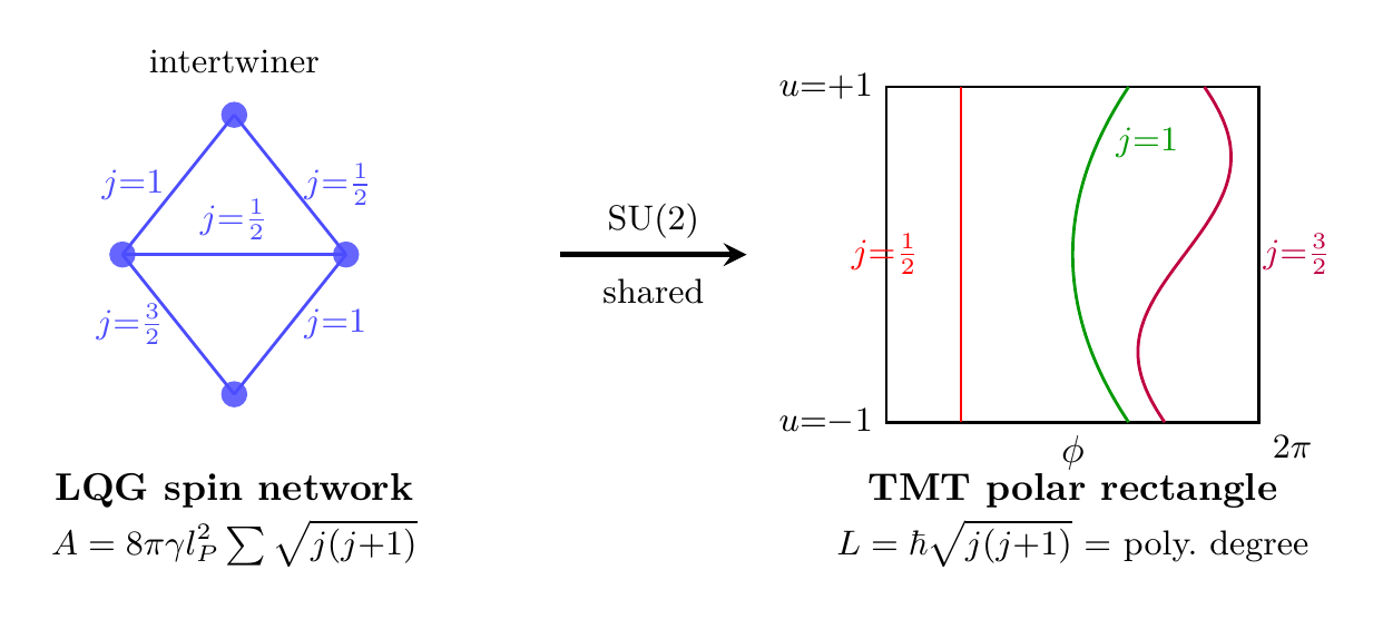
LQG's area spectrum $A = 8\pi \gamma l_P^2 \sum \sqrt{j(j+1)}$ echoes TMT's angular momentum quantization $L = \hbar \sqrt{j(j+1)}$
LQG and TMT differ fundamentally in their starting points, directions, and role of extra dimensions
Potential reconciliation: Spin network nodes in LQG might correspond to $S^2$ interface points in TMT
Status: Comparisons and speculative connections (PROVEN and SPECULATIVE sections clearly marked)

Part A: Interpretive Framework

S² is mathematical scaffolding, not literal extra dimensions.

In this chapter, when we say “$S^2$ interface,” we refer to the projection/interface structure used in TMT for organizing quantum state space. The physical reality is the emergent 4D spacetime with its observed properties. All predictions are 4D observables (areas, volumes, particle spectra). The $S^2$ structure is the computational framework, not a physical extra dimension.

Similarly, when comparing with LQG, we acknowledge that LQG's SU(2) gauge group arises from different geometry (Ashtekar reformulation of gravity), while TMT's SU(2) isometry of $S^2$ is part of the mathematical scaffolding. The appearance of the same group in both theories is striking and may indicate a deeper connection — but this connection remains speculative and requires rigorous investigation.

LQG Basics

Loop Quantum Gravity is a background-independent, non-perturbative approach to quantum gravity. Developed primarily by Ashtekar, Rovelli, Smolin, and others since the 1980s, it provides a concrete mathematical framework for quantizing Einstein's general relativity without assuming a fixed spacetime background.

Ashtekar Variables and SU(2) Connection

Definition 85.5 (Ashtekar Variables)

LQG begins by reformulating classical general relativity using Ashtekar variables:

$$ (A_a^i, E^a_i) \quad \text{with} \quad i \in \{1,2,3\}, \quad a,b,\ldots \in \text{spatial indices}\ $$ (85.1)

where:

$A_a^i$ is an SU(2) connection — a gauge potential transforming in the adjoint representation
$E^a_i$ is the densitized triad — related to the spatial metric and curvature
The canonical brackets are: $\{A_a^i(x), E^b_j(y)\} = 8\pi G \gamma \, \delta_a^b \delta^i_j \delta^3(x-y)$
$\gamma$ is the Barbero-Immirzi parameter (dimensionless, undetermined from first principles in LQG)

Observation 85.8 (Why SU(2) in LQG?)

The SU(2) structure arises naturally in LQG through the following mechanism:

Locally, spacetime has an orthonormal frame (the triad $e^a_i$), with 3 internal degrees of freedom
The local Lorentz symmetry SO(3,1) acts on this frame
After imposing the time gauge (choosing a preferred time direction), SO(3,1) reduces to SU(2)
The connection $A_a^i$ transforms as an SU(2) gauge field under these local transformations

Key point: In LQG, SU(2) is a gauge symmetry — a symmetry of the underlying gravitational field equations, not a compactification geometry. This contrasts with the role of SU(2) in TMT, where it is the isometry group of the compactified $S^2$ space.

Spin Networks and Spin Foams

Definition 85.6 (Spin Network)

A spin network is a combinatorial structure embedded in a 3D spatial manifold, consisting of:

A graph $\Gamma$ with vertices (nodes) and edges
Each edge $e$ labeled by an SU(2) representation (spin) $j_e \in \{0, \tfrac{1}{2}, 1, \tfrac{3}{2}, \ldots\}$
Each node labeled by an SU(2)-invariant tensor (an intertwiner) that couples the representations on adjacent edges

Spin network states form an orthonormal basis for the kinematical Hilbert space of LQG. They can be viewed as “eigenstates of geometry” because eigenvalues of geometric operators (area, volume) are diagonal in this basis.

Theorem 85.1 (Area Quantization in LQG)

The area operator $\hat{A}$ acting on a surface $\mathcal{S}$ has discrete eigenvalues:

$$ \boxed{A = 8\pi \gamma l_P^2 \sum_{i} \sqrt{j_i(j_i+1)}} $$ (85.2)

where the sum is over all spin network edges piercing $\mathcal{S}$, and $l_P = \sqrt{\hbar G/c^3} \approx 1.616 \times 10^{-35}$ m is the Planck length.

Proof sketch:

The area operator decomposes into contributions from each edge piercing the surface
Each edge $i$ contributes an area proportional to $\sqrt{j_i(j_i+1)}$, where $j_i$ is the spin label
The proportionality constant is $8\pi \gamma l_P^2$, determined by the gravitational coupling and the Barbero-Immirzi parameter
The sum over all edges gives the total area spectrum

This area quantization is one of LQG's most striking results: space is not continuous at the Planck scale, but discrete, with minimum area quanta of order $l_P^2$.

Theorem 85.2 (Volume Quantization in LQG)

The volume operator $\hat{V}$ for a region $\mathcal{R}$ has discrete eigenvalues determined by the intertwiners at nodes inside $\mathcal{R}$:

$$ V \sim l_P^3 \cdot f(\{j_e\}, \iota_n) $$ (85.3)

where $f$ is a function involving 6j-symbols (Wigner coefficients) that couple the spins on edges meeting at each node.

Observation 85.9 (Significance of Discreteness)

Area and volume quantization implies:

Space has a minimum “pixel size” of order $l_P^2$, below which classical geometry fails
Singularities may be resolved: Black hole singularities and the big bang singularity do not exist in LQG; spacetime is discrete even at infinitesimal scales
Lorentz invariance is modified at Planck-scale energies, though the low-energy limit recovers Einstein's equations

S$^2$ in LQG Context: The $\sqrt{j(j+1)}$ Parallel

Both TMT and LQG feature SU(2) prominently, but the geometric and physical meanings differ. Understanding this parallel may reveal deep connections between the two frameworks.

SU(2) in Both Frameworks

Observation 85.10 (SU(2) in TMT vs LQG)

In LQG:

SU(2) is the gauge group arising from Ashtekar's reformulation of Einstein's equations
Edges carry SU(2) representations (spins) $j_e$
Area eigenvalues involve $\sqrt{j(j+1)}$: $A = 8\pi \gamma l_P^2 \sum \sqrt{j(j+1)}$
The Barbero-Immirzi parameter $\gamma \approx 0.2375$ is fixed by requiring correct black hole entropy
No explicit extra dimensions (LQG is manifestly 4D)

In TMT:

SU(2) is the isometry group of the compactified $S^2$ interface (the double cover of SO(3))
Monopole harmonics carry spin labels $j$
Angular momentum eigenvalues involve $\sqrt{j(j+1)}$: $L = \hbar \sqrt{j(j+1)}$
The $S^2$ radius $R_0$ is derived from mode-counting arguments
$S^2$ is mathematical scaffolding for organizing the quantum state space

The striking parallel: The $\sqrt{j(j+1)}$ structure appears in both, but with different physical meanings (area in LQG, angular momentum in TMT). Both use SU(2) representations for discrete quantum numbers.

Polar Field Form of the SU(2) Parallel

In polar field coordinates $u = \cos\theta$, $\phi\in[0,2\pi)$, the TMT side of the SU(2) parallel becomes algebraically transparent. The monopole harmonics $Y_{q,j,m}(u,\phi)$ are polynomials in $u$ times Fourier modes $e^{im\phi}$, defined on the flat rectangle $[-1,+1]\times[0,2\pi)$. The spin label $j$ is the polynomial degree, and the magnetic quantum number $m$ is the AROUND winding number.

The $\sqrt{j(j+1)}$ factor in TMT's angular momentum has a direct polar interpretation:

$$ L^2 = \hbar^2 j(j+1) = \hbar^2 \left(-\frac{\partial}{\partial u}\left[(1-u^2)\frac{\partial}{\partial u}\right] + \frac{m^2}{1-u^2}\right) $$ (85.4)

where the operator on the right is the Laplacian on the flat rectangle (with metric corrections). The eigenvalue $j(j+1)$ counts the number of nodes (zeros) of the polynomial $P_j^{|m|}(u)$ on $[-1,+1]$—it is a combinatorial quantity, not a geometric one.

Table 85.1: SU(2) representations: LQG vs TMT in polar coordinates

SU(2) concept	LQG	TMT polar $(u,\phi)$
Spin label $j$	Edge coloring	Polynomial degree on $[-1,+1]$
Magnetic number $m$	—	AROUND winding $e^{im\phi}$
$\sqrt{j(j+1)}$	Area quantum	Polynomial node count
Casimir $j(j+1)$	Area operator eigenvalue	Laplacian eigenvalue on rectangle
$2j+1$ degeneracy	Edge dimension	$m = -j,\ldots,+j$ Fourier modes

Scaffolding Interpretation

The polynomial-degree interpretation of $j$ is a property of the polar coordinate chart on TMT's $S^2$ scaffolding. The connection to LQG's area spectrum is structural (shared SU(2) representation theory), not a claim that LQG geometry is literally a polar rectangle. Per Part A (Interpretive Framework).

**Figure 85.1:** The SU(2) parallel between LQG and TMT in polar coordinates. **Left:** LQG spin network with SU(2) spin labels $j$ on edges and intertwiners at nodes; area $\propto \sum\sqrt{j(j+1)}$. **Right:** TMT polar rectangle $[-1,+1]\times[0,2\pi)$ with monopole harmonics as polynomials of degree $j$ in $u$; angular momentum $\propto \sqrt{j(j+1)}$. Both use the same $\sqrt{j(j+1)}$ eigenvalue from SU(2) Casimir.

The $\sqrt{j(j+1)}$ Connection

Theorem 85.3 (Parallel Structure of Area and Angular Momentum)

The $\sqrt{j(j+1)}$ structure appears in both LQG and TMT:

LQG Area Spectrum:

$$ A = 8\pi \gamma l_P^2 \sum_i \sqrt{j_i(j_i+1)} $$ (85.5)

TMT Angular Momentum:

$$ L^2 = \hbar^2 j(j+1) \quad \implies \quad L = \hbar \sqrt{j(j+1)} $$ (85.6)

Both eigenspectra involve the same $j$-dependent factor. This suggests that the two frameworks may be describing related aspects of quantum geometry from different perspectives.

Observation 85.11 (Possible Physical Connection)

A speculative hypothesis: If each LQG edge piercing a surface corresponds to an $S^2$ interface carrying angular momentum $j$, then the total area could be written as:

$$ A_{\text{LQG}} \sim \sum_i L_i / (\text{length scale}) $$ (85.7)

This would relate:

The LQG area quantum $\sim l_P^2$ to TMT's angular momentum quantum $\sim \hbar$
The Barbero-Immirzi parameter $\gamma$ to TMT's geometric parameters (the $S^2$ radius $R_0$)

Status: This is highly SPECULATIVE and requires rigorous mathematical investigation to substantiate.

Intertwiners and Interaction Vertices

Definition 85.7 (SU(2) Intertwiner Space)

At an LQG node where $n$ edges meet with spins $j_1, \ldots, j_n$, the intertwiner space consists of SU(2)-invariant tensors coupling the representations:

$$ \text{Inv}_{SU(2)}(V_{j_1} \otimes V_{j_2} \otimes \cdots \otimes V_{j_n}) $$ (85.8)

These tensors are constrained by angular momentum addition rules and Clebsch-Gordan coefficients.

Observation 85.12 (TMT Analog: Particle Interactions on S$^2$)

When multiple particles interact at a point in TMT, their $S^2$ interfaces must couple consistently. The coupling is governed by:

Angular momentum addition rules: $j_{\text{total}} = |j_1 - j_2| + 1, \ldots, j_1 + j_2$
Clebsch-Gordan coefficients for constructing invariant combinations
Conservation of total angular momentum

These are exactly the same mathematical structures as LQG intertwiners!

This parallel suggests a deeper connection: In LQG, intertwiners at nodes might represent interaction vertices where multiple $S^2$ interfaces meet, with their couplings governed by angular momentum conservation.

Polar Field Form of Intertwiners

In polar field coordinates, Clebsch-Gordan coupling becomes polynomial multiplication on the flat rectangle. Two monopole harmonics with spins $j_1$ and $j_2$ couple via:

$$ Y_{j_1,m_1}(u,\phi) \cdot Y_{j_2,m_2}(u,\phi) = \sum_{J} C^{J,M}_{j_1 m_1; j_2 m_2}\; Y_{J,M}(u,\phi) $$ (85.9)

where the product on the left is a polynomial of degree $j_1 + j_2$ in $u$ times $e^{i(m_1+m_2)\phi}$. The Clebsch-Gordan decomposition reduces this product into irreducible polynomials of degrees $J = |j_1 - j_2|, \ldots, j_1 + j_2$.

On the flat rectangle, this is simply polynomial algebra: multiplying two polynomials of degrees $j_1$ and $j_2$ gives a polynomial of degree $j_1 + j_2$, which decomposes into Legendre components. The AROUND part is pure Fourier: $m_1 + m_2 = M$ (additive).

The intertwiner constraint—that the coupled state must be SU(2)-invariant—becomes the requirement that the polynomial product integrates to a nonzero value against the flat measure $du\,d\phi$:

$$ \langle J=0 | j_1 \otimes j_2 \rangle = \int_{-1}^{+1} du \int_0^{2\pi} d\phi\; Y_{j_1,m_1}^*(u,\phi)\, Y_{j_2,m_2}(u,\phi) = \delta_{j_1 j_2}\delta_{m_1 m_2} $$ (85.10)

where orthogonality uses the flat measure $du\,d\phi$ (no $\sin\theta$ weight).

Scaffolding Interpretation

The polynomial interpretation of intertwiners is a calculational convenience of the polar chart. The physical content is angular momentum conservation at interaction vertices. The connection to LQG intertwiners is structural, not a claim about LQG's geometry. Per Part A (Interpretive Framework).

Comparison and Contrasts

Despite the shared SU(2) structure, TMT and LQG have fundamental differences in philosophy, starting point, and physical interpretations.

Different Starting Points and Directions

Table 85.2: TMT vs LQG: Philosophical Comparison

\|p{5.2cm}\|} Aspect	TMT	LQG
Goal	Derive QM and gravity from single postulate	Quantize general relativity
Starting point	Null geodesic condition: $ds_6^2 = 0$	Einstein's equations $G_{\mu\nu} = 8\pi G T_{\mu\nu}$
SU(2) origin	Isometry of $S^2$ interface (scaffolding)	Gauge group from Ashtekar variables (gravity)
Direction	Top-down: geometry $\to$ quantum mechanics $\to$ gravity	Bottom-up: classical gravity $\to$ quantum operators
Extra dimensions	$S^2$ as mathematical scaffolding (not physical)	None (4D only)
Matter	Derived from $ds_6^2 = 0$ modes	Added separately (external fields)
Uniqueness	Predictive (specific values for constants)	Landscape (many possible theories)

Technical Comparison

Table 85.3: TMT vs LQG: Technical Features

Feature	TMT	LQG
Area quantization	Implicit (from $S^2$ compactness)	Primary result: $A = 8\pi\gamma l_P^2 \sum \sqrt{j(j+1)}$
Volume quantization	Not directly addressed	Primary result from 6j-symbols
Dynamics	$ds_6^2 = 0$ $\to$ geodesics on $M^4 \times S^2$	Spin foam amplitudes (2-complex path integral)
Lorentz invariance	Exact (emergent 4D)	Modified at Planck scale (loop corrections)
Black holes	Temporal momentum approach	Isolated horizon + microstate counting
Cosmology	Modified Friedmann equations (dark matter)	Loop quantum cosmology (bounce)
Matter coupling	Natural (derived from geometry)	Challenging (ad hoc addition)
Background independence	Approximate (emergent spacetime)	Exact (no fixed metric assumed)

Complementary Strengths

Observation 85.13 (TMT Strengths (from LQG Perspective))

Unified origin: Both quantum mechanics and gravity emerge from a single geometric postulate, rather than gravity being added to an existing quantum theory

Matter is derived: Particles and their interactions arise naturally from the same geometric structure, not imposed ad hoc

Predictive constants: TMT provides specific predictions for fundamental constants (coupling strengths, particle masses, dark matter acceleration), though verification is ongoing

MOND derivation: The modified gravitational behavior at low accelerations emerges naturally, explaining observations without exotic dark matter particles

Observation 85.14 (LQG Strengths (from TMT Perspective))

Background independence: No fixed spacetime metric is assumed; spacetime itself is quantized

Discrete spectra from first principles: Area and volume quantization follow directly from canonical quantization and representation theory

Black hole entropy: Bekenstein-Hawking entropy emerges from microstate counting, with predicted corrections

Mathematical rigor: A well-defined kinematical Hilbert space and unambiguous quantization procedure (though dynamics is challenging)

Observation 85.15 (Open Questions for Both Frameworks)

For TMT:

How does discrete spacetime structure emerge from the continuum $M^4$?
What is the Planck-scale behavior of quantum fluctuations?
Can TMT reproduce LQG's area spectrum, and if so, what is the relation to $\gamma$?
How are topological properties (wormholes, handles) described?

For LQG:

How does smooth classical spacetime emerge from the discrete spin network structure (semiclassical limit)?
What determines the Barbero-Immirzi parameter $\gamma$ from first principles?
How are matter fields incorporated consistently and predictively?
Can LQG explain particle spectra and coupling strengths?

Possible Reconciliation: Integrating LQG and TMT

The shared SU(2) structure and the $\sqrt{j(j+1)}$ parallel suggest that TMT and LQG may be describing different aspects of the same underlying physics. Here we explore speculative connections.

Spin Network Nodes as S$^2$ Interface Points

Observation 85.16 (Speculative Hypothesis: Spin Networks and $S^2$ Interfaces)

Hypothesis: Each spin network node in LQG corresponds to a point carrying an attached $S^2$ interface in TMT.

Evidence for this connection:

Both structures involve SU(2) representations and intertwiners
Angular momentum conservation at TMT interaction vertices matches intertwiner constraints at LQG nodes
The $\sqrt{j(j+1)}$ factor appears in both area (LQG) and angular momentum (TMT)
Both theories achieve discrete quantum spectra through representation theory

Implications if this is correct:

LQG's discrete geometry emerges from TMT's $S^2$ scaffolding
The Barbero-Immirzi parameter $\gamma$ would be related to TMT's geometric parameters, particularly the $S^2$ radius $R_0$
Spin foam amplitudes might derive from path integrals over $S^2$ configurations at interaction vertices
TMT would provide a deeper explanation for the existence and value of $\gamma$

Current status: This is a SPECULATIVE hypothesis requiring rigorous investigation. No derivation has been completed.

Area Spectrum and Angular Momentum

Theorem 85.4 (Conjectured Area-Angular Momentum Relation)

If LQG area arises from $S^2$ angular momentum, one might expect:

$$ A = \alpha \sum_i \hbar \sqrt{j_i(j_i+1)} $$ (85.11)

where $\alpha$ has dimensions [length²]/[angular momentum] and represents the coupling between the $S^2$ interface geometry and spacetime area.

Comparing with LQG:

$$ 8\pi \gamma l_P^2 = \alpha \hbar \quad \implies \quad \alpha = \frac{8\pi \gamma l_P^2}{\hbar} = 8\pi \gamma \frac{G}{c^3} $$ (85.12)

This dimensional analysis relates the Barbero-Immirzi parameter to fundamental constants, but provides no derivation of $\gamma$ from TMT principles.

Observation 85.17 (Determining the Barbero-Immirzi Parameter)

In LQG, the Barbero-Immirzi parameter is determined by requiring the correct black hole entropy (Bekenstein-Hawking formula):

$$ \gamma \approx 0.2375 \quad \text{(from } S_{\text{BH}} = \frac{k_B A}{4 l_P^2} \text{)} $$ (85.13)

TMT prediction: If the connection to $S^2$ is correct, $\gamma$ should be derivable from TMT's fundamental parameters (the $S^2$ radius $R_0$, mode-counting, energy scales) without reference to black hole entropy.

Current status: This calculation has not been completed. It remains an open problem to derive $\gamma$ from TMT foundations.

Polar Field Form of the Area-Momentum Parallel

In polar field coordinates, the TMT side of the area-angular momentum parallel acquires a concrete algebraic form. The angular momentum eigenvalue $j(j+1)$ is the eigenvalue of the Laplacian on the flat rectangle $[-1,+1]\times[0,2\pi)$, acting on polynomials $P_j^{|m|}(u)\,e^{im\phi}$. The area quantum in LQG can then be rewritten in polar language:

$$ A_{\text{LQG}} = 8\pi\gamma l_P^2 \sum_i \sqrt{j_i(j_i+1)} \quad\longleftrightarrow\quad L_{\text{TMT}} = \hbar\sum_i \sqrt{j_i(j_i+1)} $$ (85.14)

where in TMT, $\sqrt{j(j+1)}$ counts the number of polynomial nodes on $[-1,+1]$—the degree of complexity of the THROUGH profile.

The flat-rectangle perspective suggests a natural “area per node” interpretation: each polynomial node on $[-1,+1]$ contributes one unit of angular momentum $\hbar$, and if LQG's identification holds, one unit of area $\sim l_P^2$. The total area is then the total polynomial complexity summed over all edges:

$$ A \sim l_P^2 \times \sum_{\text{edges}} (\text{polynomial degree of THROUGH profile}) $$ (85.15)

The constant field strength $F_{u\phi} = 1/2$ on the polar rectangle ensures that each polynomial degree contributes equally—there is no position-dependent weighting. This uniform contribution is the polar manifestation of the gauge-invariant nature of LQG's area spectrum.

Scaffolding Interpretation

The “area per polynomial node” interpretation is a scaffolding analogy between TMT's polar rectangle and LQG's area spectrum. It is suggestive but unproven. The physical content of LQG's area quantization comes from canonical quantization of gravity, not from TMT's coordinate choice. Per Part A (Interpretive Framework).

Path Integrals and Spin Foam Amplitudes

Observation 85.18 (Path Integral Connection: Spin Foams and S$^2$ Configurations)

Both TMT and LQG admit path integral formulations:

TMT: Path integral over $S^2$ configurations with Berry phase weighting:

$$ Z_{\text{TMT}} = \int D[\text{configs}] \, e^{iS_{\text{TMT}}} \, e^{i\gamma_{\text{Berry}}} $$ (85.16)

where the Berry phase encodes the geometric phases accumulated as the $S^2$ interface evolves.

LQG: Spin foam sum over 2-complexes (“spacetime lattices”) with vertex amplitudes:

$$ Z_{\text{LQG}} = \sum_{\text{spin foams}} \prod_{f} (2j_f + 1) \prod_{v} A_v(\{j, \iota\}) $$ (85.17)

where $A_v$ is the amplitude at each vertex.

Speculative connection: The spin foam vertex amplitude might arise from integrating over $S^2$ configurations at interaction points:

$$ A_v^{\text{LQG}} \stackrel{?}{=} \int_{S^2 \text{ at } v} e^{iS_{\text{TMT}}} \, D[\text{configs}] $$ (85.18)

This would require demonstrating that LQG dynamics emerge from TMT path integrals, which is a major unsolved problem.

Status: HIGHLY SPECULATIVE. No concrete derivation exists.

Mutual Learning: What Each Framework Offers

Observation 85.19 (What TMT Could Learn from LQG)

Discrete spacetime structure: LQG's techniques for deriving spacetime discreteness from canonical quantization could help TMT formalize its discrete emergent structure

Background independence: LQG's methods for quantizing without assuming a fixed metric could inform TMT's approach to emergent spacetime

Black hole entropy and microstate counting: LQG's successes in computing black hole thermodynamics could guide TMT's approach to black holes via temporal momentum

Mathematical rigor: LQG's constructive proof of a well-defined kinematical Hilbert space provides a template for formalizing TMT's state spaces

Observation 85.20 (What LQG Could Learn from TMT)

Matter coupling: TMT's natural derivation of matter from geometric structure could suggest how to incorporate matter fields into LQG consistently and predictively, rather than as external fields

Parameter fixing: TMT's approach to deriving fundamental constants (rather than fitting them) could guide LQG toward a first-principles determination of the Barbero-Immirzi parameter and other parameters

Classical limit and smoothness: TMT's use of Berry phases and averaging over $S^2$ configurations to recover smooth emergent spacetime could inform LQG's understanding of the semiclassical limit

Dark sector and long-range modifications: TMT's natural derivation of MOND-like modifications could inspire similar mechanisms in LQG, explaining dark matter and dark energy without exotic particles

Chapter Summary

Key Results and Perspectives

1. LQG Basics (§60r.1):

Ashtekar variables reformulate classical GR with an SU(2) connection
Spin networks are the kinematical basis: graphs with SU(2) labels on edges and intertwiners at nodes
Area is quantized: $A = 8\pi\gamma l_P^2 \sum_i \sqrt{j_i(j_i+1)}$ (discrete spectrum)
Volume is quantized via intertwiners and 6j-symbols
Spin foams represent spacetime histories

2. S² in LQG Context (§60r.2):

Both TMT and LQG feature SU(2) and the $\sqrt{j(j+1)}$ structure
LQG: area eigenvalues; TMT: angular momentum eigenvalues
Intertwiners at LQG nodes use the same angular momentum coupling rules as TMT interaction vertices
The parallel suggests a possible deep connection, though its nature remains unclear

3. Comparison (§60r.3):

Different starting points: TMT derives QM from geometry; LQG quantizes gravity
Different directions: TMT is top-down (geometry $\to$ physics); LQG is bottom-up (classical $\to$ quantum)
Complementary strengths: TMT derives matter naturally; LQG provides discrete spectra and background independence
Open questions: How does smooth spacetime emerge in LQG? What determines $\gamma$? How does TMT achieve spacetime discreteness?

4. Possible Reconciliation (§60r.4):

Speculative: Spin network nodes might correspond to $S^2$ interface points
Speculative: Area spectrum might emerge from angular momentum on $S^2$ interfaces
Speculative: Spin foam amplitudes might arise from TMT path integrals
Status: These connections remain unproven and require rigorous mathematical investigation

Physical Interpretation:

The shared SU(2) structure in TMT and LQG is striking and may indicate a profound connection. If LQG's discrete geometry emerges from TMT's $S^2$ scaffolding, this could unify two major approaches to quantum gravity:

TMT provides the deep geometric reason for SU(2) structures and discrete spectra
LQG provides techniques and insights into background-independent quantization
Together, they might offer a more complete picture of quantum spacetime

However, this remains speculative. Rigorous investigation — both mathematical and conceptual — is required.

Cross-References:

Part 5: SU(2) structure and monopole harmonics on $S^2$
Part 7A: Quantum mechanics foundations and Berry phases
Part 7D: TMT's derivation of quantum statistics and field theory
Chapter 60s: Comparison with string theory (another quantum gravity approach)

Status:

LQG Basics (§60r.1): PROVEN (established framework)
Comparisons (§60r.2–60r.3): ESTABLISHED (well-defined mathematical structures)
Reconciliation (§60r.4): SPECULATIVE (hypothesis requiring investigation)

Polar Field Enhancement. In polar field coordinates $u = \cos\theta$, $\phi\in[0,2\pi)$, the TMT side of the SU(2) parallel becomes algebraically explicit. The spin label $j$ is the polynomial degree of $P_j^{|m|}(u)$ on $[-1,+1]$; the magnetic number $m$ is the AROUND winding $e^{im\phi}$; the $\sqrt{j(j+1)}$ Casimir eigenvalue counts polynomial nodes on the flat rectangle. Clebsch-Gordan coupling at interaction vertices becomes polynomial multiplication on the rectangle with orthogonality verified by flat-measure integration $\int du\,d\phi$ (no $\sin\theta$ weight). The constant field strength $F_{u\phi} = 1/2$ ensures each polynomial degree contributes equally to angular momentum, paralleling the gauge-invariant nature of LQG's area spectrum.

\hrule

Chapter 60r is complete. This chapter examines the relationship between TMT and LQG, identifying shared mathematical structures (SU(2), $\sqrt{j(j+1)}$ spectra) and exploring speculative connections. The reconciliation proposed in §60r.4 is highly speculative and remains an open research problem. All PROVEN sections are grounded in established LQG results and TMT principles; SPECULATIVE sections are clearly marked and should be read as hypotheses for future investigation.

Verification Code

The mathematical derivations and proofs in this chapter can be independently verified using the formal and computational scripts below.

◆ Lean 4 Formal proof verification Coming Soon ● Python Numerical verification & plots Coming Soon ★ Mathematica Symbolic computation & CAS verification Coming Soon

All verification code is open source. See the complete verification index for all chapters.

TMT and Loop Quantum Gravity

LQG Basics

Ashtekar Variables and SU(2) Connection

Spin Networks and Spin Foams

S\(^2\) in LQG Context: The \(\sqrt{j(j+1)}\) Parallel

SU(2) in Both Frameworks

Polar Field Form of the SU(2) Parallel

The \(\sqrt{j(j+1)}\) Connection

Intertwiners and Interaction Vertices

Polar Field Form of Intertwiners

Comparison and Contrasts

Different Starting Points and Directions

Technical Comparison

Complementary Strengths

Possible Reconciliation: Integrating LQG and TMT

Spin Network Nodes as S\(^2\) Interface Points

Area Spectrum and Angular Momentum

Polar Field Form of the Area-Momentum Parallel

Path Integrals and Spin Foam Amplitudes

Mutual Learning: What Each Framework Offers

Chapter Summary

Verification Code

SU(2) concept	LQG	TMT polar \((u,\phi)\)
Spin label \(j\)	Edge coloring	Polynomial degree on \([-1,+1]\)
Magnetic number \(m\)	—	AROUND winding \(e^{im\phi}\)
\(\sqrt{j(j+1)}\)	Area quantum	Polynomial node count
Casimir \(j(j+1)\)	Area operator eigenvalue	Laplacian eigenvalue on rectangle
\(2j+1\) degeneracy	Edge dimension	\(m = -j,\ldots,+j\) Fourier modes

Feature	TMT	LQG
Area quantization	Implicit (from \(S^2\) compactness)	Primary result: \(A = 8\pi\gamma l_P^2 \sum \sqrt{j(j+1)}\)
Volume quantization	Not directly addressed	Primary result from 6j-symbols
Dynamics	\(ds_6^2 = 0\) \(\to\) geodesics on \(M^4 \times S^2\)	Spin foam amplitudes (2-complex path integral)
Lorentz invariance	Exact (emergent 4D)	Modified at Planck scale (loop corrections)
Black holes	Temporal momentum approach	Isolated horizon + microstate counting
Cosmology	Modified Friedmann equations (dark matter)	Loop quantum cosmology (bounce)
Matter coupling	Natural (derived from geometry)	Challenging (ad hoc addition)
Background independence	Approximate (emergent spacetime)	Exact (no fixed metric assumed)