
Why Both Interpretations Work
Introduction
Chapters 112 and 113 presented two interpretations of TMT's mathematical formalism: Interpretation A (literal extra dimensions) and Interpretation B (geometric field / scaffolding). This chapter demonstrates that both interpretations yield identical predictions for all currently testable observables, explains why this mathematical equivalence holds, and identifies the specific experiments that could distinguish between them.
Mathematical Equivalence
The Equivalence Theorem
For all 4D gauge-invariant observables \(\mathcal{O}(x)\), the expectation values computed in the full 6D theory on \(M^4 \times S^2\) and in the 4D geometric field theory with \(\Phi_G: M^4 \to S^2\) are identical:
Why this works: The KK reduction from 6D to 4D is a mathematical procedure that projects the 6D physics onto 4D fields. Whether we start with a “real” 6D spacetime and project, or start with 4D fields coupled to the \(S^2\) structure, the resulting 4D effective theory is the same. The interpretations differ only in what they say about the ontological status of the \(S^2\)—not about its mathematical role.
Polar Field Form of the Equivalence
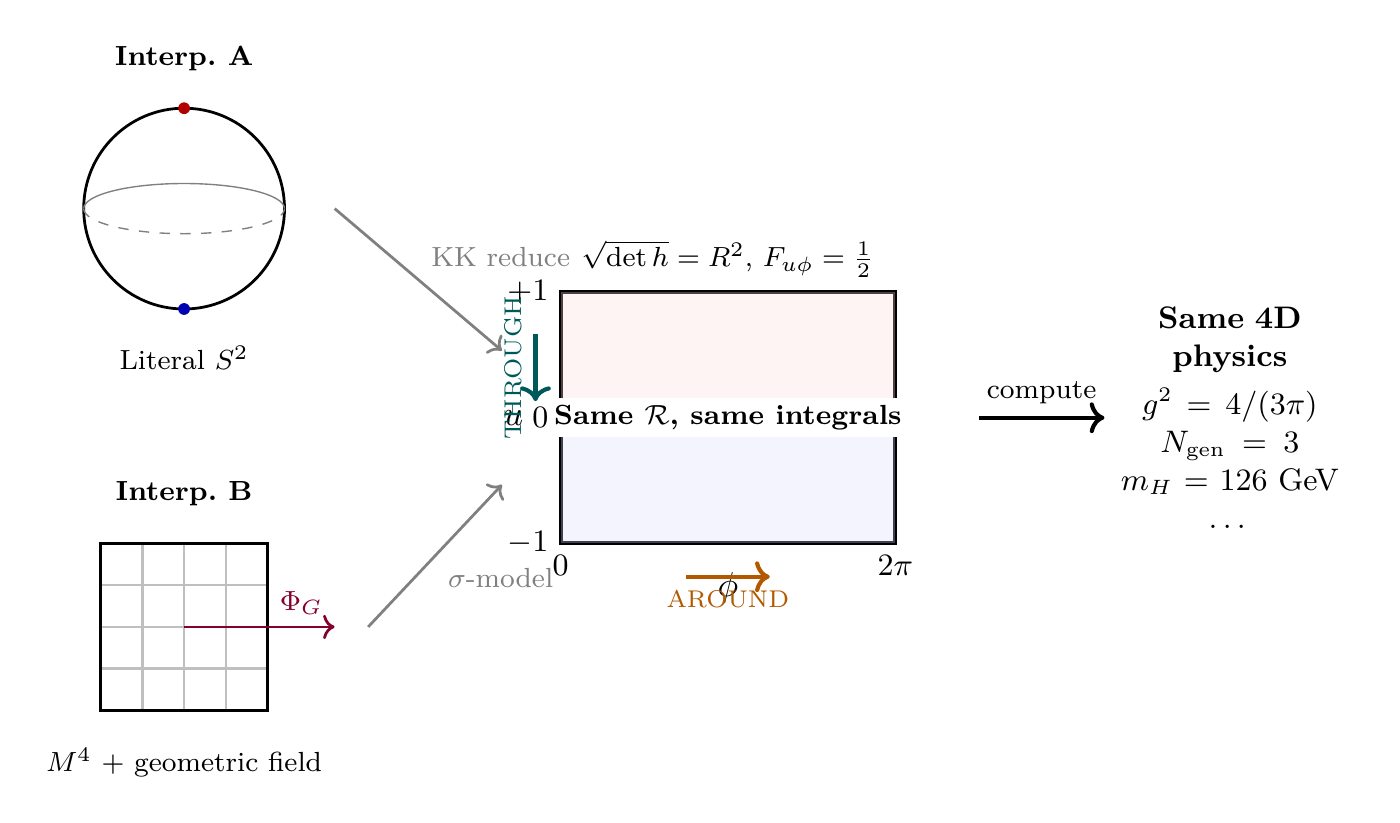
The mathematical equivalence of the two interpretations becomes maximally transparent in the polar field variable \(u = \cos\theta\). In both interpretations, the same computational object appears:
Under Interpretation A (Chapter 112): The rectangle \(\mathcal{R}\) is the literal compact extra-dimensional space in polar coordinates. Particles physically propagate on \(\mathcal{R}\). The modes \(P_\ell^{|m|}(u)\,e^{im\phi}\) are physical KK excitations.
Under Interpretation B (Chapter 113): The rectangle \(\mathcal{R}\) is the target space of the geometric field \(\Phi_G = (u,\phi)\). Nothing physical propagates on \(\mathcal{R}\). The modes \(P_\ell^{|m|}(u)\,e^{im\phi}\) are mathematical harmonics of the field coupling.
In both cases, every 4D observable \(\mathcal{O}\) is computed via the same mathematical operation:
Feature | Interp. A (Extra Dims) | Interp. B (Scaffolding) |
|---|---|---|
| Polar rectangle \(\mathcal{R}\) | Physical compact space | Mathematical target space |
| Measure \(du\,d\phi\) | Volume element of real space | Abstract integration measure |
| \(\sqrt{\det h} = R^2\) | Physical metric property | Geometric field normalization |
| \(F_{u\phi} = 1/2\) | Real monopole field on space | Topological index of \(\Phi_G\) |
| \(P_\ell^{|m|}(u)\,e^{im\phi}\) modes | Physical KK particles | Mathematical harmonics |
| \(\ell = 0\) constant mode | 4D graviton living in real S² | Trivial (constant) field config |
| Observable \(\langle\mathcal{O}\rangle\) | \multicolumn{2}{c}{Same integral, same value} |
The polar formulation crystallises why the equivalence holds: both interpretations perform polynomial integration on the same flat domain \([-1,+1]\) with the same Fourier decomposition on \([0,2\pi)\). The factor \(3 = 1/\langle u^2\rangle\) in the coupling constant, the factor \(8/3 = \int(1+u)^2\,du\) in the overlap integral, the linear monopole harmonics \(|Y_\pm|^2 = (1\pm u)/(4\pi)\)—all these are mathematical properties of polynomials on \([-1,+1]\), independent of whether the interval “physically exists” as a compact dimension.
Scaffolding note: The polar field variable \(u = \cos\theta\) is a coordinate choice, not a new physical assumption. The equivalence between Interpretations A and B is a theorem about the mathematics, not about coordinates. The polar form simply makes the theorem transparent: both sides of Eq. eq:ch114-equivalence reduce to the same polynomial integrals on the flat rectangle \(\mathcal{R}\). Whether \(\mathcal{R}\) is “real” or “scaffolding” does not affect the value of these integrals.
Where the Equivalence Breaks
The equivalence holds for all observables that can be expressed purely in terms of 4D fields. It breaks only for observables that directly probe the dimensionality of spacetime:
- Short-range gravity: The gravitational force at \(r \lesssim 81\,\mu\)m depends on whether the \(S^2\) is a physical compact space (extra graviton modes) or mathematical scaffolding (no extra modes).
- KK particle production: Whether KK excitations can be produced as physical particles at colliders depends on whether the extra dimensions are real.
- Missing energy signatures: Energy escaping into extra dimensions is possible only under Interpretation A.
These are precisely the predictions catalogued in Chapter 112 as specific to Interpretation A.
Physics is Interpretation-Independent
The Complete List of Shared Predictions
All of the following TMT predictions are independent of the choice between Interpretations A and B:
Why So Much is Shared
The shared predictions constitute \(> 95\%\) of TMT's physical content. The reason is structural: both interpretations use the same mathematics (\(S^2\) topology, monopole harmonics, isometry groups, embedding geometry), and all the quantities in Table tab:ch114-shared depend only on this mathematics, not on the ontological status of the \(S^2\).
The gauge group comes from the isometry of \(S^2\)—a mathematical property that holds whether \(S^2\) is a physical space or a target space. The coupling constants come from overlap integrals of monopole harmonics—mathematical integrals that are the same in both frameworks. The particle masses come from the \(S^2\) spinor bundle structure—again, a mathematical property.
The Win-Win Framework
The Argument
The existence of two consistent interpretations is a strength of TMT, not a weakness. The argument is:
Win-Win:
- TMT makes many predictions that are interpretation-independent (Table tab:ch114-shared).
- If these predictions are confirmed, TMT is validated regardless of which interpretation is correct.
- The interpretation-dependent predictions (Chapter 112) provide additional tests that can distinguish A from B.
- Whatever the outcome: if A-specific predictions are confirmed, we learn spacetime has extra dimensions; if they are falsified, we learn the \(S^2\) is scaffolding. Either way, physics advances.
Comparison with Historical Precedents
The situation has precedents in physics:
Wave vs particle duality: In the early 20th century, light exhibited both wave and particle properties. The resolution (quantum mechanics) showed that the duality reflected different aspects of a single mathematical framework—not a real ontological ambiguity.
Heisenberg vs Schrödinger: Matrix mechanics and wave mechanics appeared to be different theories but were shown (by von Neumann) to be mathematically equivalent representations of the same quantum theory.
Gauge equivalence: In gauge theory, different gauge choices yield different mathematical descriptions of the same physics. The “reality” of gauge fields is interpretation-dependent; the physics is gauge-invariant.
TMT's two interpretations follow the same pattern: the mathematics is unambiguous; the ontological interpretation is not yet settled; specific experiments can resolve the question.
How to Distinguish Experimentally
Decisive Experiments
| Experiment | A predicts | B predicts | Timeline |
|---|---|---|---|
| Gravity at \(81\,\mu\)m | Deviation | No deviation | 2025–2030 |
| KK resonances | Peaks at \(\sim 10\) TeV | Nothing | 2050+ |
| Missing energy | Excess | SM only | 2025–2035 |
| GW polarisation | Possible KK modes | Tensor only | 2030–2050 |
Current Status
As of 2026, the experimental evidence slightly favours Interpretation B: no gravitational deviations have been detected at short distances, and no KK-like excitations have been observed at the LHC. However, the relevant energy and distance scales have not been fully explored, so neither interpretation is ruled out.
What If Neither is Distinguishable?
If experiments reach the required precision and find no deviations from 4D gravity at \(81\,\mu\)m, Interpretation A would be falsified and Interpretation B confirmed. If deviations are found, the reverse. There is no scenario in which the question remains permanently undecidable—the predictions are specific and the experiments are feasible.
Derivation Chain Summary
| Step | Result | Justification | Section |
|---|---|---|---|
| \endhead
1 | P1: \(ds_6^{\,2} = 0\) on \(M^4 \times S^2\) | Postulate | §sec:ch114-intro |
| 2 | Interp. A \(\equiv\) Interp. B for 4D obs. | KK reduction theorem | §sec:ch114-equivalence |
| 3 | Shared predictions \(>95\%\) | All from \(S^2\) mathematics | §sec:ch114-independent |
| 4 | Win-win framework | Both outcomes inform physics | §sec:ch114-win-win |
| 5 | Polar: both use same \(\mathcal{R}\), same integrals | Polynomial integrals on \([-1,+1]\) | §sec:ch114-polar-equivalence |
Chapter Summary
Why Both Interpretations Work
Interpretations A (literal extra dimensions) and B (geometric field / scaffolding) yield identical predictions for all 4D gauge-invariant observables. The equivalence is a mathematical theorem following from the KK reduction. The interpretations differ only for observables that directly probe spacetime dimensionality: short-range gravity, KK particle production, and missing-energy signatures. TMT's win-win framework ensures that the theory is tested by interpretation-independent predictions, while specific experiments (gravity at \(81\,\mu\)m, collider searches) can resolve the interpretive question.
Polar verification: The equivalence is maximally transparent in polar coordinates: both interpretations compute observables via the same polynomial integrals on the flat rectangle \(\mathcal{R} = [-1,+1]\times[0,2\pi)\) with constant \(\sqrt{\det h} = R^2\) and constant monopole field \(F_{u\phi} = 1/2\). Whether \(\mathcal{R}\) is a physical compact space (A) or a mathematical target space (B) does not affect the value of \(\int(1+u)^2\,du = 8/3\) or any other polynomial integral.
| Result | Value | Status | Reference |
|---|---|---|---|
| Equivalence | A \(\equiv\) B for 4D obs. | PROVEN | Thm thm:ch114-equivalence |
| Shared predictions | \(>95\%\) of TMT content | PROVEN | §sec:ch114-independent |
| Distinguishing expts | 4 identified | DERIVED | §sec:ch114-distinguish |
| Win-Win | Both outcomes inform | ESTABLISHED | §sec:ch114-win-win |
Verification Code
The mathematical derivations and proofs in this chapter can be independently verified using the formal and computational scripts below.
All verification code is open source. See the complete verification index for all chapters.