Chapter 2

The Single Postulate

Roadmap

This chapter introduces the single postulate of Temporal Momentum Theory and derives its immediate consequences. We begin with the null constraint $ds_6^{\,2} = 0$ and show how this equation, together with the observed properties of our universe (position-independent masses, 4D Lorentz covariance, and the vacuum definition), forces the mathematical framework into a product structure $\mathcal{M}^4 \times S^2$, establishes a velocity budget $v^2 + v_T^2 = c^2$, and reveals that mass is temporal momentum: $p_T = mc/\gamma$. The key physical insight is that $E = mc^2$ is not an independent fact of nature — it is a consequence of the velocity budget at rest. By the end of this chapter, you will understand (1) what P1 asserts and what it does not, (2) why the product structure is forced by P1 combined with observed physics, (3) how mass arises as temporal momentum, and (4) why no alternative to P1 produces a viable theory.

Prerequisites: Familiarity with special relativity (Lorentz factor, four-vectors), basic differential geometry (metrics, geodesics), and linear algebra. No quantum field theory is assumed.

Main results: The null constraint Eq. eq:ch2-P1, velocity budget Eq. eq:ch2-velocity-budget, product structure Theorem thm:P1-Ch2-product-structure, temporal momentum Eq. eq:ch2-temporal-momentum-def, rest energy Eq. eq:ch2-emc2-from-pT, and uniqueness Theorem thm:P1-Ch2-counterfactual.

Key diagrams: Figure fig:ch2-null-decomposition-balance (null decomposition balance), Figure fig:ch2-product-structure-bundle (product structure), Figure fig:ch2-temporal-momentum-concept (temporal momentum), Figure fig:ch2-derivation-chain-flowchart (chapter derivation chain).

Statement of P1: $ds_6^{\,2} = 0$

Every physical theory rests on postulates — assumptions taken as starting points from which everything else follows. Newton's mechanics rests on three laws. Special relativity rests on the constancy of $c$ and the equivalence of inertial frames. General relativity rests on the equivalence principle. Quantum mechanics rests on the Hilbert space structure and Born's rule.

Temporal Momentum Theory rests on one postulate.

Postulate 2.4 (P1 — The Null Constraint)

The conservation structure governing massive particles satisfies the null constraint:

$$ \boxed{ds_6^{\,2} = 0 \quad \text{for all massive particles}} $$ (2.1)

where the six-dimensional mathematical framework employs the line element:

$$ ds_6^{\,2} = g_{AB} \, dx^A dx^B $$ (2.2)

Here $g_{AB}$ is a pseudo-Riemannian metric tensor (symmetric, non-degenerate, with signature $(-,+,+,+,+,+)$: Lorentzian in the 4D sector and positive-definite on the $S^2$ projection structure), and the indices $A, B \in \{0, 1, 2, 3, 5, 6\}$ range over all six dimensions of the scaffolding framework.

Remark 2.5 (Anticipatory Notation)

The subscript “6” in $ds_6^{\,2}$ is anticipatory notation. P1 properly states $ds_D^2 = 0$ on $\mathcal{M}^4 \times K^{D-4}$ for some dimension $D$. That $D = 6$ — and that $K^2 = S^2$ is the unique compact internal manifold — is not assumed but derived from P1 together with the requirements of non-abelian gauge symmetry, stability, and topological charge quantization (Chapter 3, Theorem 3.1: The Dimension Theorem). We write $ds_6^{\,2}$ throughout for readability, with the understanding that this notation encodes a result proven in the next chapter.

This single equation is the entire postulational content of TMT. Every result derived in Parts I through XI — every particle mass, every coupling constant, every cosmological parameter — traces back to Eq. eq:ch2-P1 and nothing else.

Scaffolding Interpretation

Foundational Interpretation: P1 does NOT assert that particles literally travel through a six-dimensional space. The six-dimensional mathematics is scaffolding — a computational framework encoding the conservation structure of temporal momentum.

The constraint $ds_6^{\,2} = 0$ encodes the fundamental conservation relationship between spatial motion (in $\mathcal{M}^4$) and temporal momentum (on the $S^2$ projection structure). The Tesseract Framework (see Core Principles \S19) provides the conceptual picture for understanding this conservation: 3D space (inner cube), 4D temporal momentum (outer cube), gravity connecting them (edges). The framework is a structured way of thinking about what P1 means physically — not a second principle. The $S^2$ that emerges is projection structure, not hidden space. “6D” is a mathematical framework, not an ontological claim.

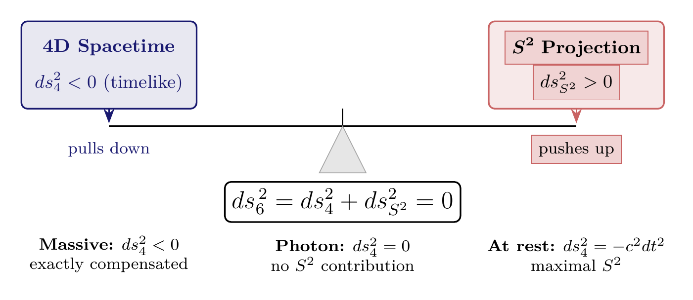
In words: The null constraint $ds_6^{\,2} = 0$ says that every massive particle “moves” at speed $c$ through the full conservation structure. The 4D spacetime interval ($ds_4^2 < 0$, timelike) is exactly compensated by the internal projection contribution ($ds_{S^2}^2 > 0$). This is a conservation law: the total “velocity” through the mathematical framework is always $c$, and it is partitioned between spatial motion and temporal motion on the projection structure.

Physical Picture: The Null Constraint: A Perfectly Balanced Ledger

Imagine a particle carrying a fixed “velocity account” of exactly $c$. This account has two columns: spatial velocity (how fast the particle moves through space) and temporal velocity (how fast it moves through time). The null constraint says the total across both columns is always $c$ — no more, no less. A particle sitting still puts everything in the temporal column. A particle moving close to the speed of light transfers nearly everything to the spatial column. But the sum never changes. This is not a metaphor layered on top of the physics — it IS the physics. The mathematical equation $ds_6^{\,2} = 0$ is precisely this bookkeeping rule, expressed in the language of geometry.

Historical context: The idea that higher-dimensional mathematics might encode physical forces dates to Theodor Kaluza (1921) and Oskar Klein (1926), who showed that a fifth dimension could unify gravity and electromagnetism. TMT extends this program to six dimensions but differs fundamentally in interpretation: the extra mathematics is scaffolding for a conservation law, not a claim about hidden spatial dimensions. The null constraint $ds_6^{\,2} = 0$ is TMT's distinctive contribution — Kaluza-Klein theory uses timelike geodesics ($ds_5^2 < 0$), not null ones.

What the Postulate Asserts

In standard relativity, there is a fundamental asymmetry between massive and massless particles:

Massless particles (photons): $ds^2 = 0$ (null geodesics in 4D)
Massive particles: $ds^2 < 0$ (timelike geodesics in 4D)

P1 asserts that this asymmetry is an artifact of viewing physics in four dimensions alone. When the full conservation structure is considered — mathematically represented in a six-dimensional framework — all particles satisfy the null constraint. The difference between massive and massless particles is not a difference in kind, but a difference in how the null constraint distributes between observable (4D) and internal ($S^2$) degrees of freedom.

Theorem 2.1 (Universal Null Character — P1 Decomposed)

This is not an independent result — it is P1 itself, decomposed into 4D and $S^2$ contributions using the product structure $\mathcal{M}^4 \times S^2$ (Theorem thm:P1-Ch2-product-structure).

Every particle in nature — massive or massless — satisfies $ds_6^{\,2} = 0$. For massive particles, the 4D timelike character ($ds_4^2 < 0$) is exactly compensated by the $S^2$ projection contribution ($ds_{S^2}^2 > 0$):

$$ \underbrace{ds_4^2}_{< 0 \text{ (timelike in 4D)}} + \underbrace{ds_{S^2}^2}_{> 0 \text{ (projection contribution)}} = 0 $$ (2.3)

For massless particles ($m = 0$), the velocity budget gives $v_T = 0$ (since all of $c$ is allocated to spatial velocity $v = c$), so the $S^2$ contribution $ds_{S^2}^2 = v_T^2 \, dt^2 = 0$ vanishes, and $ds_4^2 = 0$ recovers the standard 4D null condition. This exact cancellation is illustrated as a balance in Figure fig:ch2-null-decomposition-balance.

**Figure 2.1:** The null decomposition from P1: the 4D timelike contribution ($ds_4^2 < 0$) and the $S^2$ projection contribution ($ds_{S^2}^2 > 0$) exactly cancel for every particle. Massive particles have both contributions nonzero and balanced; photons have no $S^2$ contribution; particles at rest allocate maximum contribution to the $S^2$ projection structure. (Eq. eq:ch2-null-decomposition)

This is not a derived result — it IS P1, restated in decomposed form. The physical content is the velocity budget, derived as follows.

We now derive the velocity budget — the central kinematic consequence of P1. The question we are answering is: if the total 6D interval vanishes, what constraint does this impose on a particle's spatial velocity $v$ and its rate of change on the $S^2$ projection structure? The derivation is short (four equations) and proceeds by dividing the null constraint by $dt^2$ and identifying each term. Watch for the moment when the constraint becomes $v^2 + v_T^2 = c^2$ — this simple equation is the Pythagorean-like partition that underlies all of special relativity.

Derivation of the velocity budget from P1. Consider a massive particle moving through the 6D scaffolding framework. We derive the velocity budget first in flat spacetime ($g_{\mu\nu} = \eta_{\mu\nu}$, $h_{ij} = R_0^2 \hat{h}_{ij}$); the general curved-spacetime case replaces $v^2$ with the physical velocity $g_{ij} dx^i dx^j / dt^2$ and follows identically.

Along the particle's worldline, parameterized by coordinate time $t$, the 6D line element is:

$$ ds_6^2 = g_{\mu\nu} \, dx^\mu dx^\nu + h_{ij} \, d\xi^i d\xi^j $$ (2.4)

\stepnote{Starting point: $ds_6^2$ split into 4D + $S^2$ sectors.}

Dividing by $dt^2$:

$$ \frac{ds_6^2}{dt^2} = g_{\mu\nu} \frac{dx^\mu}{dt} \frac{dx^\nu}{dt} + h_{ij} \frac{d\xi^i}{dt} \frac{d\xi^j}{dt} $$ (2.5)

\stepnote{Divided both sides by $dt^2$; each term is now a squared velocity.}

Caution: Coordinate Time vs. Proper Time

We parameterize by coordinate time $t$, not proper time $\tau$. Dividing by $dt^2$ gives velocities $dx^\mu/dt$ measured in coordinate time. Using proper time instead would introduce an extra factor of $\gamma^2$ (since $d\tau = dt/\gamma$) and obscure the simple Pythagorean structure of the result. The coordinate-time parameterization is what makes the velocity budget $v^2 + v_T^2 = c^2$ manifest.

In flat spacetime with signature $(-+++)$ and $x^0 = ct$:

$$ \eta_{\mu\nu} \frac{dx^\mu}{dt} \frac{dx^\nu}{dt} = -\left(\frac{dx^0}{dt}\right)^2 + \delta_{ij}\frac{dx^i}{dt}\frac{dx^j}{dt} = -c^2 + v^2 $$ (2.6)

\stepnote{Expanded $\eta_{\mu\nu}$; used $dx^0/dt = c$ and defined $v^2$.} where $dx^0/dt = c$, and $v^2 \equiv \delta_{ij}(dx^i/dt)(dx^j/dt)$ is the squared magnitude of the ordinary three-velocity in flat space. Define the temporal velocity:

$$ v_T^2 \equiv h_{ij} \frac{d\xi^i}{dt} \frac{d\xi^j}{dt} $$ (2.7)

\stepnote{Defined $v_T^2$ as the $S^2$ sector contribution.} which is the squared magnitude of the rate of change of the $S^2$ projection coordinates with respect to coordinate time.

Substituting into P1 ($ds_6^2 = 0$):

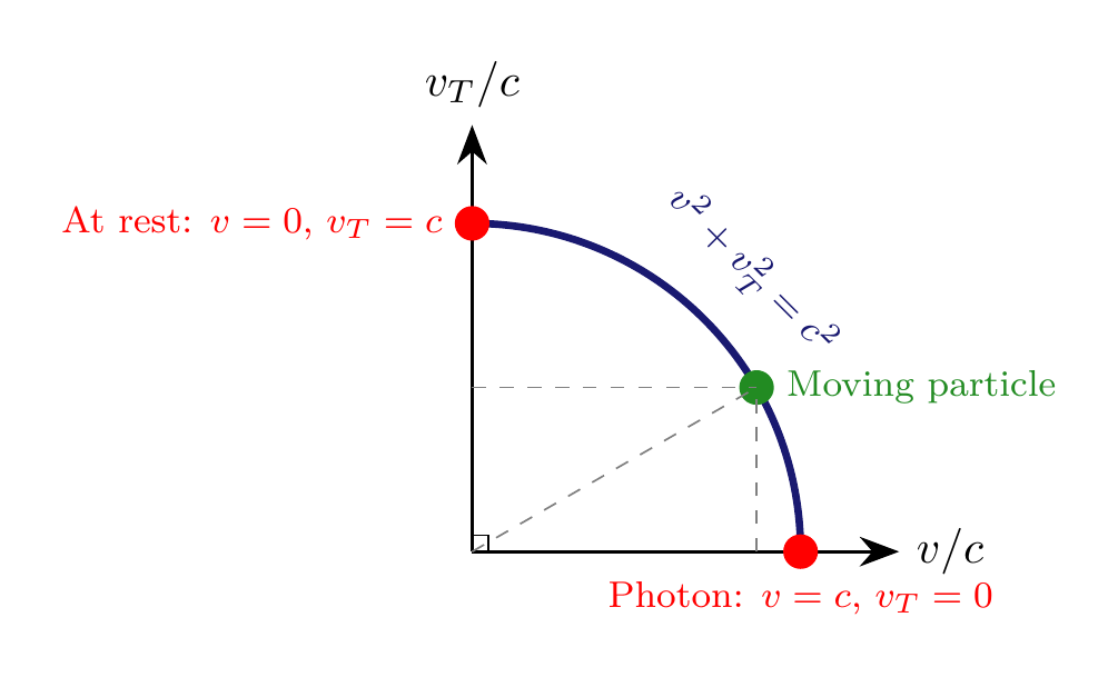
$$ \frac{ds_6^2}{dt^2} = -(c^2 - v^2) + v_T^2 = 0 \quad \Longrightarrow \quad \boxed{v^2 + v_T^2 = c^2} $$ (2.8)

\stepnote{Set $ds_6^2/dt^2 = 0$ (P1); rearranged to velocity budget.}

In words: Every particle has a total “speed budget” of $c$, shared between ordinary spatial velocity $v$ and temporal velocity $v_T$. A particle at rest ($v = 0$) moves entirely through time at speed $c$. A photon ($v = c$) has no temporal velocity at all. For any intermediate speed, spatial and temporal motion trade off on a quarter circle — gaining speed in space means losing speed through time. This is time dilation, expressed as a velocity partition.

Analogy: Analogy: Fixed-Balance Bank Account

The velocity budget works like a bank account with a fixed total balance of $c$. You have two sub-accounts: “spatial velocity” and “temporal velocity.” You can transfer funds between them, but the total balance never changes. Depositing more into the spatial account (accelerating through space) automatically withdraws from the temporal account (slowing down through time). The constraint $v^2 + v_T^2 = c^2$ is the balance equation.

Where the analogy holds:

The total is conserved: you cannot create or destroy velocity, only redistribute it.
Extremes are well-defined: all-spatial (photon) and all-temporal (at rest).
Transfer is continuous: you can smoothly move between extremes.

Where it breaks down:

Bank accounts add linearly ($a + b = c$), but velocities add in quadrature ($v^2 + v_T^2 = c^2$). The quarter-circle constraint surface is not a straight line. This quadrature arises from the Pythagorean structure of the metric (see the “Why Not?” box below).
The “temporal” sub-account does not correspond to a literal velocity through a hidden space; it is a mathematical encoding of the time-dilation factor.

Why Not: Why Not $v + v_T = c$ Instead of $v^2 + v_T^2 = c^2$?

You might expect a linear budget: spatial velocity plus temporal velocity equals $c$. But the null constraint $ds_6^{\,2} = 0$ involves the metric, which measures squared intervals. When you divide $ds_6^2 = 0$ by $dt^2$, you get a sum of squared velocities — not a sum of velocities — because the metric is a quadratic form in the coordinate differentials. The quadrature relation $v^2 + v_T^2 = c^2$ is geometrically a quarter circle (Pythagorean theorem in velocity space), not a straight line. This is not a choice; it is forced by the Riemannian structure of the mathematics. A linear constraint $v + v_T = c$ would require a fundamentally different (non-metric) geometry that is incompatible with special relativity's invariance structure.

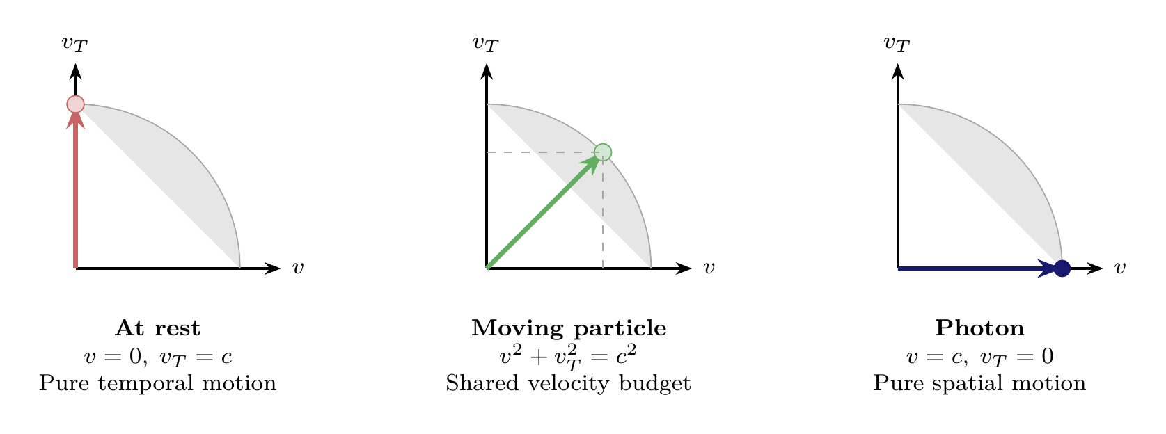
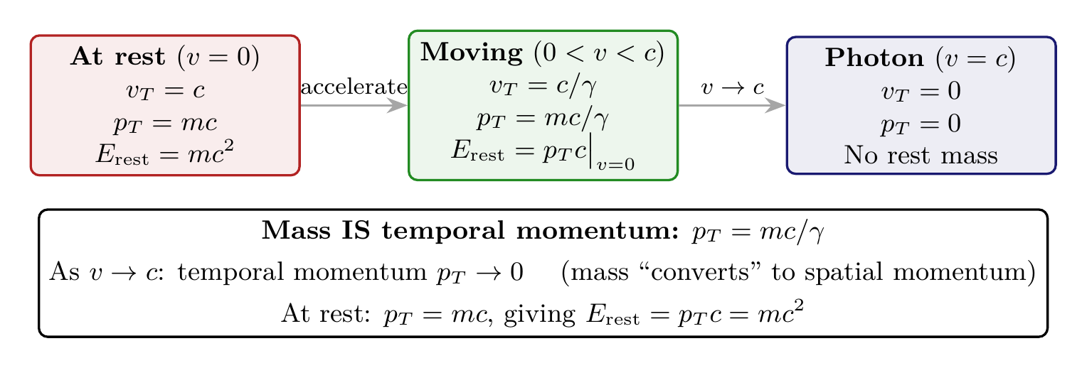
Every particle partitions its “total velocity” $c$ between ordinary spatial velocity $v$ and temporal velocity $v_T$. The three limiting cases are:

At rest ($v = 0$): $v_T = c$ — the particle moves purely through time.
Photon ($v = c$): $v_T = 0$ — all velocity is spatial, with no temporal component. The $S^2$ projection contribution vanishes, recovering the standard 4D null condition $ds_4^2 = 0$.
Intermediate: $v$ and $v_T$ trade off in quadrature on the quarter circle $v^2 + v_T^2 = c^2$.

These three cases are depicted side by side in Figure fig:ch2-three-limiting-cases.

Thought Experiment: What If the Speed Budget Were Larger Than $c$?

Suppose the velocity budget were $v^2 + v_T^2 = C^2$ for some $C > c$. Then a particle at rest would have temporal velocity $v_T = C > c$, meaning it would “move through time” faster than light. The rest energy would be $E_{\text{rest}} = mC^2$ — larger than $mc^2$. The speed of light in vacuum would still be $c$ (set by the electromagnetic field's dispersion relation), but the fundamental velocity scale of the conservation structure would be $C$. This would break the exact identification between the velocity budget and special relativity's time dilation: $d\tau/dt = v_T/C \neq v_T/c$. The Lorentz factor would no longer control time dilation. Special relativity as we know it would fail. The fact that the budget is exactly $c$ — the same $c$ that appears in electrodynamics — is not coincidental. It is a consistency requirement: the conservation structure and the propagation of massless particles must share the same fundamental velocity.

**Figure 2.2:** Three limiting cases of the velocity budget $v^2 + v_T^2 = c^2$. Left: a particle at rest allocates all velocity to temporal motion ($v_T = c$). Center: a moving massive particle shares the budget between spatial and temporal components. Right: a photon allocates all velocity to spatial motion ($v = c$), with zero temporal velocity. The gray quarter circle shows the constraint surface. (Eq. eq:ch2-velocity-budget)

The Vocabulary of P1

Several terms in the statement of P1 require precise definition:

Table 2.1: Key terms in P1 and their precise meanings

Term	Precise Meaning
“Conservation structure”	The mathematical framework encoding how energy, momentum, and mass interrelate. Not a literal space.
“$ds_6^{\,2}$”	The line element in the six-dimensional scaffolding framework $\mathcal{M}^4 \times S^2$.
“Null constraint”	The condition $ds_6^{\,2} = 0$, stating that the 4D and $S^2$ contributions exactly cancel.
“Massive particles”	All particles with rest mass $m > 0$: electrons, quarks, neutrinos, $W$, $Z$, Higgs.
“Scaffolding”	The 6D mathematics is a computational tool, not a claim about the number of spatial dimensions.
“Velocity budget”	The constraint $v^2 + v_T^2 = c^2$: every particle partitions the universal speed $c$ between spatial velocity $v$ and temporal velocity $v_T$.
“Temporal momentum”	The momentum associated with temporal velocity: $p_T = mv_T = mc/\gamma$. Equal to $mc$ at rest; vanishes for photons.

The velocity budget established the physical picture: every particle shares the universal speed $c$ between spatial and temporal motion. We now turn to the mathematical machinery that makes this precise — the null constraint expressed in momentum space, the product structure it forces, and the equations of motion that follow.

Mathematical Form of the Null Geodesic Hypothesis

In this section, we express P1 in momentum space, derive the product structure $\mathcal{M}^4 \times S^2$ from the null constraint, develop the polar field representation, and obtain the geodesic equation. These mathematical tools are the foundation for every derivation in the rest of the book.

The Null Constraint in Momentum Space

For a particle described in the 6D scaffolding framework with six-momentum $k^A$ (the generalized momentum conjugate to $x^A$; for a massive particle, $k^A$ has dimensions of momentum [kg$\cdot$m/s] and reduces to the standard four-momentum $p^\mu$ in the 4D sector), P1 states:

$$ k^A k_A = g_{AB} \, k^A k^B = 0 $$ (2.9)

The product structure $\mathcal{M}^4 \times S^2$ (Theorem thm:P1-Ch2-product-structure; treated in full generality in Chapter 4) decomposes this into 4D and $S^2$ projection parts:

$$ g_{\mu\nu} k^\mu k^\nu + h_{ij} k^i k^j = 0 $$ (2.10)

where:

$g_{\mu\nu}$ is the 4D metric with signature $(-+++)$
$h_{ij}$ is the positive-definite metric on the $S^2$ projection structure
Greek indices $\mu, \nu = 0, 1, 2, 3$ label 4D coordinates
Latin indices $i, j = 5, 6$ label $S^2$ projection coordinates

The first term is negative (timelike in 4D for massive particles), the second is positive (definite on $S^2$). The null constraint requires these to exactly cancel:

$$ \underbrace{g_{\mu\nu} k^\mu k^\nu}_{< 0 \text{ (4D timelike)}} + \underbrace{h_{ij} k^i k^j}_{> 0 \text{ ($S^2$ projection)}} = 0 $$ (2.11)

In words: In momentum language, a massive particle's 4D momentum is timelike (its squared norm is negative), while its $S^2$ projection momentum is spacelike (positive-definite). The null constraint forces these two contributions to cancel exactly. The magnitude of the $S^2$ projection momentum is $mc$ — the particle's rest mass times the speed of light — so mass is directly encoded in the internal momentum.

Physical Picture: Why Masses Are Discrete: Vibrations on a Drum

Picture a circular drumhead. When you strike it, it vibrates — but not at any arbitrary frequency. The drumhead's boundary forces the vibrations into specific allowed patterns (modes), each with a definite frequency. The smaller the drum, the higher the lowest frequency; the shape of the drum determines which frequencies are allowed. The $S^2$ projection structure plays exactly this role for particle masses. The compact geometry of $S^2$ acts like the boundary of a drum, and the allowed “vibration modes” of the internal momentum correspond to the allowed masses. Compactness is what makes the spectrum discrete: an infinite, non-compact surface would allow vibrations at any frequency — a continuous mass spectrum, which contradicts the fact that particles have definite, isolated masses.

Remark 2.6 (Compactness of $K^2$)

The internal manifold $K^2$ must be compact. This is not an additional assumption but a consequence of P1: the null constraint $ds_6^{\,2} = 0$ requires the $S^2$ momentum components $k^i$ to satisfy $h_{ij} k^i k^j = -g_{\mu\nu} k^\mu k^\nu > 0$, which for a particle of mass $m$ gives $h_{ij} k^i k^j = m^2 c^2$.

Upon quantization, the internal momentum components $k^i$ are no longer free parameters but are determined by the eigenvalue problem for the Laplace-Beltrami operator $\Delta_{K^2}$ on the internal manifold: $\Delta_{K^2} Y_n = -\lambda_n Y_n$, where the eigenvalues $\lambda_n$ (with dimensions $1/\text{length}^2$) determine the allowed masses via $m_n^2 c^2 = \hbar^2 \lambda_n$ (equivalently, $m_n = \hbar \sqrt{\lambda_n}/c$). For the mass spectrum to be discrete (as observed — particles have definite, isolated masses rather than a continuous distribution), this eigenvalue problem must have a discrete spectrum.

By the spectral theorem for the Laplace-Beltrami operator on Riemannian manifolds: compact manifolds have purely discrete spectra (a consequence of the Rellich-Kondrachov compactness theorem, which ensures that the resolvent of $\Delta_{K^2}$ is a compact operator), while non-compact manifolds generically have continuous essential spectra. Therefore $K^2$ must be compact. Non-compact $K^2$ would produce a continuous mass spectrum, contradicting observation.

The specific identification $K^2 = S^2$ follows from the additional requirements of stability, non-abelian gauge symmetry (the isometry group of $S^2$ is $SO(3)$, which is non-abelian; the torus $T^2$ has isometry group $U(1) \times U(1)$, which is abelian and gives only abelian gauge structure), and topological charge quantization ($\pi_2(S^2) = \mathbb{Z}$ supports magnetic monopole configurations; $\pi_2(T^2) = 0$ does not), as derived in Chapter 3.

The Product Structure

The null constraint does not merely describe propagation on an assumed background — together with the observed properties of particles in our universe, it forces the mathematical framework to decompose into a product structure.

Caution: What the product structure requires beyond P1

The null constraint $ds_6^{\,2} = 0$ alone admits null curves on metrics far more general than direct products. Consider a general 6D metric $g_{AB}(x,\xi)$ with positive-definite internal block $h_{ij}$. For any timelike 4D tangent $u^\mu$ (with $g_{\mu\nu}u^\mu u^\nu < 0$), the quadratic equation $h_{ij}w^i w^j + 2g_{\mu i}u^\mu w^i + g_{\mu\nu}u^\mu u^\nu = 0$ has at least one real solution $w^i$ (because $h_{ij}$ is positive definite and the constant term is negative). Null curves therefore exist on a far broader class of manifolds than direct products.

What forces the product structure is P1 together with the following observed properties of our universe: (i) particle masses are position-independent constants, (ii) 4D Lorentz covariance holds in the observable sector, and (iii) the vacuum is the ground state with no gauge excitations. These are not additional postulates on the same logical level as P1 — they are observational facts that any viable theory must reproduce. The proof below makes explicit which step uses which input.

Theorem 2.2 (Vacuum Product Structure from P1 and Observed Physics)

\leavevmode\newline

P1 ($ds_6^{\,2} = 0$), together with the observed position-independence of particle masses, 4D Lorentz covariance, and the definition of the vacuum as the gauge-trivial ground state, forces the decomposition of the 6D scaffolding framework into a vacuum product structure:

$$ M^6 = \mathcal{M}^4 \times K^2 $$ (2.12)

where $K^2$ is a compact 2-manifold. In the vacuum (ground state), the product is direct (unwarped). The specific identification $K^2 = S^2$ is derived in Chapter 3.

Proof.

The proof proceeds in three steps. Each step is labeled with the input it uses: P1 itself, or one of the three observational inputs stated in the theorem.

Derivation Roadmap

Derivation roadmap (3 steps):

Show that position-independent masses require the internal metric to depend only on internal coordinates, and 4D covariance requires the 4D metric to depend only on spacetime coordinates [uses: observed physics]
Eliminate 4D–internal cross-terms by identifying them as gauge fields and taking the vacuum (ground state) [uses: vacuum definition]
Show that the warp factor must be constant (position-independent masses force $f(x) = R_0$), yielding a direct product $\mathcal{M}^4 \times K^2$ [uses: P1 + observed physics]

Step 1: Position-independent masses and 4D covariance force a two-sector decomposition. [Input: observed physics — constant particle masses and Lorentz covariance.]

Consider the most general 6D metric on a manifold with 4 non-compact and 2 compact dimensions:

$$ ds_6^2 = g_{\mu\nu}(x,\xi) \, dx^\mu dx^\nu + 2 \, g_{\mu i}(x,\xi) \, dx^\mu d\xi^i + h_{ij}(x,\xi) \, d\xi^i d\xi^j $$ (2.13)

where $x^\mu$ are 4D coordinates and $\xi^i$ are internal coordinates. P1 requires $ds_6^2 = 0$ for all massive particles. This forces the metric into separable sectors, by the following argument.

Math Reminder: Kaluza-Klein Dimensional Reduction

In a Kaluza-Klein framework, a field $\Phi(x,\xi)$ on $M^4 \times K^2$ is expanded in harmonics of the internal space: $\Phi(x,\xi) = \sum_n \phi_n(x) Y_n(\xi)$, where $Y_n$ are eigenfunctions of the Laplace-Beltrami operator on $K^2$: $\Delta_{K^2} Y_n = -\lambda_n Y_n$. Each mode $\phi_n(x)$ then appears as a 4D field with mass $m_n^2 c^2 = \hbar^2 \lambda_n$. This procedure is analogous to Fourier decomposition on a circle, generalized to curved compact manifolds.

Upon Kaluza-Klein reduction, the 4D mass spectrum is determined by the eigenvalues of the internal Laplace-Beltrami operator $\Delta_{K^2}$ constructed from $h_{ij}$: a 6D field $\Phi(x,\xi)$ is expanded in internal harmonics $Y_n(\xi)$ satisfying $\Delta_{K^2} Y_n = -\lambda_n Y_n$, and each mode appears in 4D as a field of mass $m_n^2 c^2 = \hbar^2 \lambda_n$. For these masses to be constants — the same everywhere in spacetime, as observed — the eigenvalue problem $\Delta_{K^2} Y_n = -\lambda_n Y_n$ must be independent of the 4D position $x^\mu$. This requires $h_{ij} = h_{ij}(\xi)$ only, with no $x^\mu$ dependence.

Conversely, after integrating the 6D Einstein-Hilbert action over $K^2$, the effective 4D gravitational coupling and cosmological constant are determined by integrals of the form $\int_{K^2} \sqrt{h} \, d^2\xi$. For 4D general covariance to hold (the effective 4D action must depend only on $x^\mu$ through $g_{\mu\nu}(x)$ and its derivatives), the internal metric $h_{ij}$ and the 4D metric $g_{\mu\nu}$ must decouple: $g_{\mu\nu} = g_{\mu\nu}(x)$ only.

Together, these requirements force the vacuum metric into a block structure where $g_{\mu\nu}$ depends only on $x^\mu$ and $h_{ij}$ depends only on $\xi^i$, with at most a position-dependent overall scale (warp factor).

Step 2: The vacuum definition eliminates cross-terms. [Input: vacuum definition — ground state with no gauge excitations.]

The cross-terms $g_{\mu i} \, dx^\mu d\xi^i$ mix 4D and internal coordinates. In the Kaluza-Klein framework (Appendix C), these cross-terms are identified with gauge potentials: $g_{\mu i} = A_\mu^a(x) K_a^i(\xi)$, where $K_a^i$ are Killing vectors on $K^2$. The vacuum is defined as the configuration with no gauge fields excited ($A_\mu^a = 0$), giving $g_{\mu i} = 0$. This is not an additional assumption — it is the definition of the ground state about which all excitations (gauge fields, matter fields) are defined. With $g_{\mu i} = 0$, the metric separates:

$$ ds_6^2 = g_{\mu\nu}(x) \, dx^\mu dx^\nu + h_{ij}(x,\xi) \, d\xi^i d\xi^j $$ (2.14)

Checkpoint (Step 2 of 3): We have eliminated the cross-terms by recognizing them as gauge potentials and taking the vacuum configuration $A_\mu^a = 0$. The metric now splits cleanly into a 4D sector and an internal sector. What remains is to show the two sectors cannot be “warped” — i.e., the internal scale must be constant.

Step 3: P1 plus position-independent masses force a direct (unwarped) product in the vacuum. [Input: P1 ($ds_6^{\,2} = 0$) + observed position-independence of masses.]

The most general separated vacuum metric allows a warp factor:

$$ ds_6^2 = g_{\mu\nu}(x) \, dx^\mu dx^\nu + f(x)^2 \, \hat{h}_{ij}(\xi) \, d\xi^i d\xi^j $$ (2.15)

Caution: Warped vs. Direct Product

A warped product $ds_6^2 = g_{\mu\nu} dx^\mu dx^\nu + f(x)^2 \hat{h}_{ij} d\xi^i d\xi^j$ and a direct product (with $f = \text{const}$) look similar but are physically very different. A position-dependent warp factor $f(x)$ makes particle masses vary with location, because the eigenvalues of $f(x)^2 \hat{h}_{ij}$ depend on $x^\mu$. This would mean an electron in one galaxy has a different mass than an electron in another — which is ruled out observationally. The distinction matters: many string-theory constructions use warped products (Randall-Sundrum, flux compactifications), but TMT's null constraint forces the product to be direct.

where $f(x)$ is the warp factor (modulus field). P1 requires $ds_6^2 = 0$, which gives:

$$ g_{\mu\nu} k^\mu k^\nu + f(x)^2 \, \hat{h}_{ij} k^i k^j = 0 $$ (2.16)

For the mass spectrum $m^2 \propto \hat{h}_{ij} k^i k^j$ to be position-independent (an observed particle has the same mass everywhere in spacetime), the warp factor must be constant: $f(x) = R_0 = \text{const}$. A position-dependent $f(x)$ would make particle masses vary with spacetime location, violating the equivalence principle and contradicting observation.

This constancy is not merely a consistency requirement — it is dynamically enforced. The modulus field $\Phi(x) \equiv f(x) - R_0$ satisfies an effective potential $V_{\text{eff}}(\Phi)$ derived from the 6D Einstein equations. Intuitively, quantum corrections from short-distance (UV/Planck-scale) physics generate a contribution to $V_{\text{eff}}$ that grows as $R \to 0$ (resisting collapse of the compact space), while the cosmological horizon (IR) contribution grows as $R \to \infty$ (resisting unbounded expansion). The competition between these two effects produces a unique stable minimum at $f = R_0$, with $R_0$ determining the characteristic scale $L_\mu \approx 81\,\mu\text{m}$ (derived in Chapter 4, \S4.9; the full stabilization mechanism including the explicit form of $V_{\text{eff}}$ is derived in Part II, Chapter 13). Excitations $\Phi(x) \neq 0$ about this minimum correspond to a massive scalar field (the modulus), not to the vacuum.

With $f = R_0 = \text{const}$ and $g_{\mu i} = 0$, the vacuum metric is:

$$ ds_6^2 = g_{\mu\nu}(x) \, dx^\mu dx^\nu + R_0^2 \, \hat{h}_{ij}(\xi) \, d\xi^i d\xi^j $$ (2.17)

which is the metric of a direct product $\mathcal{M}^4 \times K^2$ with $K^2$ having radius $R_0$. The null constraint then gives:

$$ \underbrace{g_{\mu\nu} k^\mu k^\nu}_{= -m^2 c^2 \text{ (4D mass shell)}} + \underbrace{R_0^2 \, \hat{h}_{ij} k^i k^j}_{= +m^2 c^2 \text{ ($K^2$ eigenvalue)}} = 0 $$ (2.18)

In words: The 4D mass of every particle is determined by the eigenvalue spectrum of the compact space $K^2$. The left term is the standard mass-shell relation ($-m^2 c^2$), and the right term is the contribution from the internal geometry ($+m^2 c^2$). Their cancellation is P1: the 6D interval is null. Since the eigenvalues of a compact manifold are discrete, the particle mass spectrum is automatically discrete — no continuous range of masses is allowed.

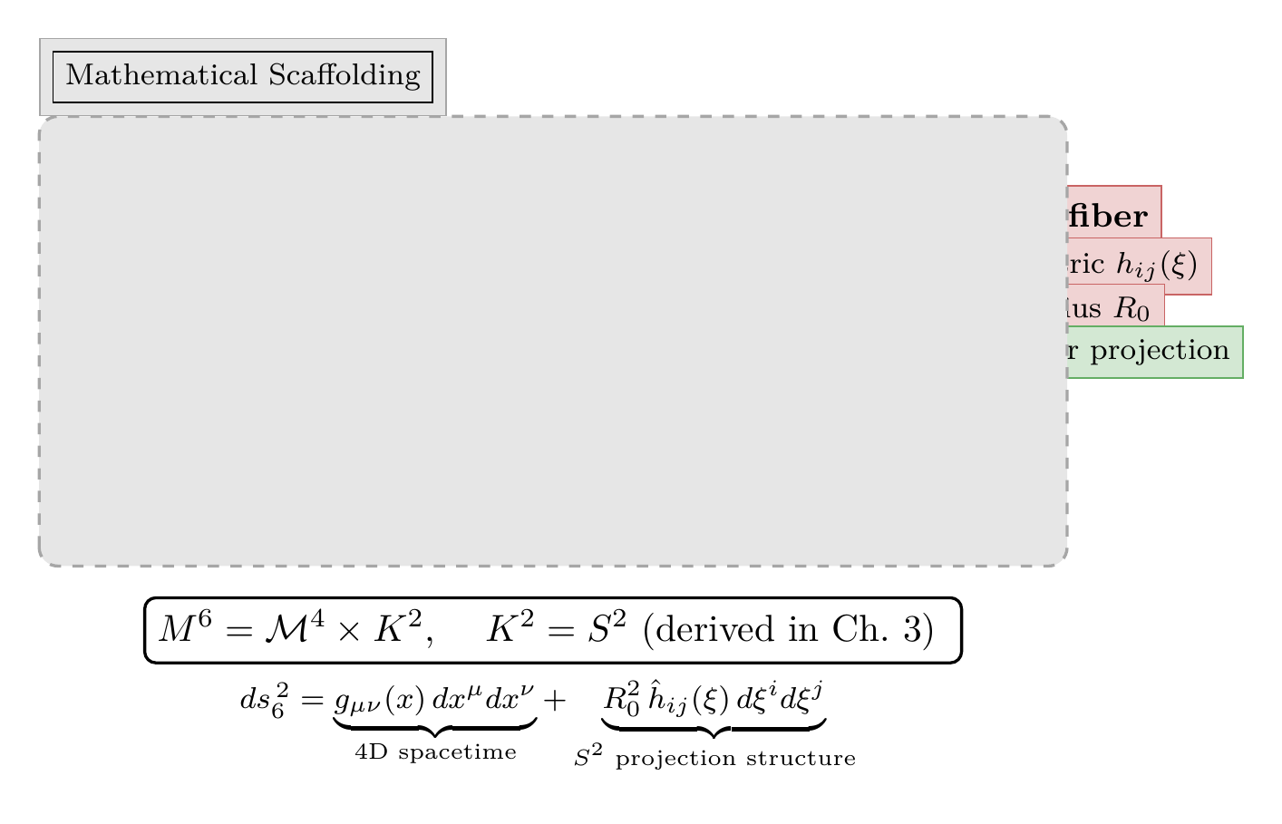
establishing that 4D mass is determined by the $K^2$ eigenvalue spectrum, as required. The product structure is visualized in Figure fig:ch2-product-structure-bundle.

The identification $K^2 = S^2$ (rather than any other compact 2-manifold) follows from three requirements, each derived from P1: (i) stability under small perturbations ($S^2$ is the unique maximally symmetric compact 2-manifold), (ii) non-abelian gauge symmetry (the isometry group $SO(3)$ of $S^2$ gives non-abelian gauge structure; the torus $T^2$ gives only $U(1) \times U(1)$, which is abelian), and (iii) topological charge quantization ($\pi_2(S^2) = \mathbb{Z}$ supports magnetic monopole configurations required for charge quantization). These are derived in Chapter 3. □

(See: Part I, \Ssec:ch2-product-structure; Part II, Chapter 13 (modulus stabilization); Chapters 3, 8 ($D=6$ uniqueness; $K^2 = S^2$ identification)) □

Why Not: Why Not Just Four Dimensions?

You might wonder: if we want to describe physics, why introduce a six-dimensional framework at all? Four dimensions work perfectly well for general relativity. The reason is that four dimensions alone cannot explain why particles have the masses they do. In 4D, particle masses are free parameters — numbers that must be measured, not calculated. The null constraint $ds_6^{\,2} = 0$ on a product $\mathcal{M}^4 \times K^2$ turns mass into an eigenvalue of the internal geometry. The mass spectrum becomes as calculable as the vibrational frequencies of a drum. Four dimensions cannot do this because there is no “internal geometry” to generate the spectrum. The extra mathematical structure is the minimum needed to make masses predictable rather than arbitrary.

Analogy: Analogy: Compass Needles at Every Point

The product structure $\mathcal{M}^4 \times K^2$ works like a compass at every point on a map. The map is 4D spacetime ($\mathcal{M}^4$), and at each point, the compass needle can point in various directions on a sphere ($S^2$). The compass direction at each point is independent of the map coordinates — this is the product structure. Moving through spacetime changes the compass reading according to definite rules (the geodesic equation and gauge transformations), but the sphere of possible readings is the same everywhere. The particle's mass is determined by how the compass “vibrates” (which eigenmode of $S^2$ it occupies), while the compass's orientation encodes gauge charges.

Where the analogy holds:

At each spacetime point, there is an independent internal structure ($S^2$).
The internal structure has the same geometry everywhere (product, not warped).
The way a particle “sits” on the internal structure determines its properties.

Where it breaks down:

A real compass has a preferred direction (magnetic north); $S^2$ has no preferred point, reflecting gauge invariance.
The $S^2$ is not a physical space — it is projection structure encoding conservation laws. The compass analogy risks suggesting a hidden physical dimension.

Summary: The product structure $\mathcal{M}^4 \times K^2$ is not assumed — it is forced by P1 together with three observational facts about our universe: constant masses demand that the internal metric depend only on internal coordinates, 4D covariance demands that the 4D metric depend only on spacetime coordinates, and position-independent masses demand that the warp factor be constant. The null constraint alone admits solutions on far more general geometries (as noted in the caution box above), but P1 combined with the observed properties of particles leaves no alternative to the product structure. The result is a clean decomposition where 4D mass is determined by the eigenvalue spectrum on $K^2$. As we will see in Chapter 3, the specific identification $K^2 = S^2$ then follows from gauge symmetry and topological requirements. Figure fig:ch2-product-structure-bundle visualizes this structure.

**Figure 2.3:** Vacuum product structure $M^6 = \mathcal{M}^4 \times S^2$ forced by P1 together with observed physics (position-independent masses, 4D covariance, vacuum definition). The 4D spacetime $\mathcal{M}^4$ (blue, bottom) serves as the base manifold, with $S^2$ fibers (red spheres) attached at each point. The dashed boundary marks this as mathematical scaffolding — a computational framework, not physical extra dimensions. The direct product metric decomposes the 6D line element into independent 4D and $S^2$ contributions. (Theorem thm:P1-Ch2-product-structure, Eq. eq:ch2-direct-product-metric)

The 6D Metric

The 6D metric takes the block-diagonal form in the vacuum configuration:

$$ ds_6^{\,2} = g_{\mu\nu}(x) \, dx^\mu dx^\nu + h_{ij}(\xi) \, d\xi^i d\xi^j $$ (2.19)

where $g_{\mu\nu}$ is the 4D metric and $h_{ij}$ is the metric on the $S^2$ projection structure with coordinates $\xi^i = (\theta, \phi)$.

The Polar Field Representation

The $S^2$ metric in the standard spherical coordinates $(\theta, \phi)$ is:

$$ h_{ij}\, d\xi^i d\xi^j = R_0^2\bigl(d\theta^2 + \sin^2\theta\, d\phi^2\bigr) $$ (2.20)

This representation, while standard, carries a coordinate-dependent weight factor $\sin\theta$ in every integral over $S^2$. The polar field representation introduces the variable $u \equiv \cos\theta$, $u \in [-1, +1]$, which absorbs this weight factor and yields a flat integration measure.

In the polar variable, the $S^2$ metric becomes:

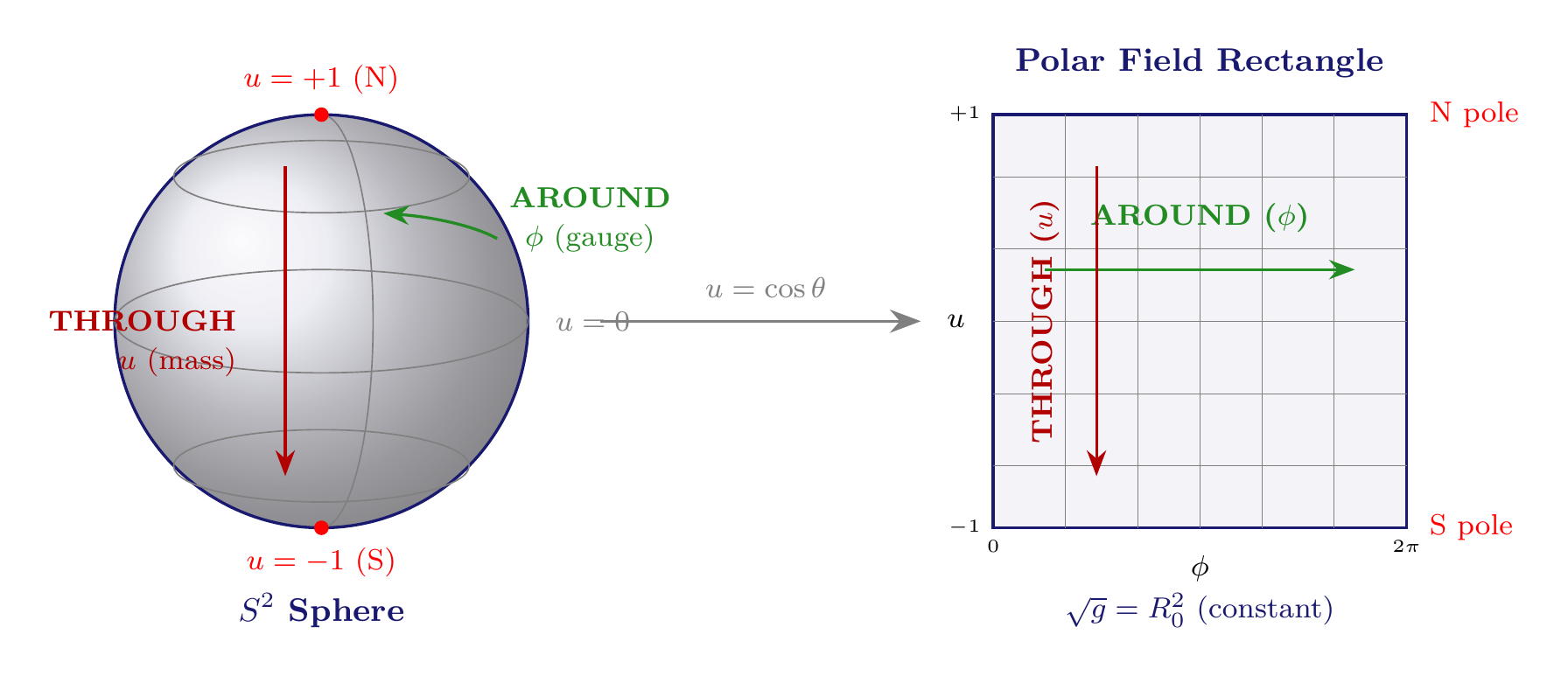
$$ \boxed{h_{ij}\, d\xi^i d\xi^j = R_0^2\left(\frac{du^2}{1 - u^2} + (1 - u^2)\, d\phi^2\right)} $$ (2.21)

In words: The variable $u = \cos\theta$ replaces the polar angle $\theta$ and absorbs the $\sin\theta$ weight that normally complicates spherical integrals. In the polar field representation, the sphere looks like a flat rectangle $[-1, +1] \times [0, 2\pi)$ with a position-dependent metric. The poles ($u = \pm 1$) appear as the top and bottom edges of the rectangle. Every integration over $S^2$ in TMT becomes a flat integral over this rectangle — no angular weight factors.

with a key property: the metric determinant is constant:

$$ \sqrt{\det h} = R_0^2, \qquad d\Omega = du\, d\phi $$ (2.22)

Every integral over $S^2$ in TMT therefore reduces to a flat integral over the rectangle $[-1, +1] \times [0, 2\pi)$. The $\sin\theta$ weight that complicates spherical-coordinate integrals is not present.

The full 6D line element in the polar field representation is:

$$ ds_6^{\,2} = g_{\mu\nu}(x)\, dx^\mu dx^\nu + R_0^2\left(\frac{du^2}{1 - u^2} + (1 - u^2)\, d\phi^2\right) $$ (2.23)

The P1 null constraint $ds_6^{\,2} = 0$ in this representation cleanly separates the $S^2$ contribution into two independent one-dimensional structures:

The polar ($u$) direction: controls mass spectra, monopole localization, and gravitational coupling (“through” physics)
The azimuthal ($\phi$) direction: controls gauge symmetry, charge conservation, and Berry phase (“around” physics)

This Around/Through factorization, derived from the separability of monopole harmonics in $(u, \phi)$, is developed fully in Chapters 9–12 and provides the structural explanation for why gauge forces (topology, “around”) and mass/gravity (dynamics, “through”) are governed by independent geometric mechanisms on the same $S^2$.

Physical Picture: Around and Through: Two Independent Highways on a Sphere

Picture the $S^2$ projection structure as a globe. There are two fundamentally different ways to move on a globe: around it (following latitude lines, circling the poles) and through it (moving from pole to pole along meridians). These two types of motion are geometrically independent — going around does not affect your north-south position, and moving through does not change your longitude. In TMT, these two directions control completely different physics. The “around” direction ($\phi$) governs gauge symmetry — how charges are assigned, how forces are transmitted, and why charge is conserved. The “through” direction ($u = \cos\theta$) governs mass and gravity — the eigenvalue spectrum that determines particle masses and the coupling to the gravitational field. This separation is not approximate; it is exact, arising from the mathematical separability of the equations on $S^2$.

Scaffolding Interpretation

Dual verification: Throughout this book, key results are derived in both the standard $(\theta, \phi)$ and polar field $(u, \phi)$ representations. The two representations are related by $u = \cos\theta$ and produce identical physical results. The dual approach serves as an independent cross-check and reveals the geometric structure behind numerical factors: for instance, the factor 3 in the interface coupling $g^2 = 4/(3\pi)$ is identified as $1/\langle u^2 \rangle_{S^2} = 1/(1/3) = 3$, the reciprocal of the second moment of the polar variable over the sphere (Chapter 20).

Remark 2.7 (Block-Diagonal Form is the Vacuum Definition)

The absence of cross-terms $g_{\mu i} \, dx^\mu d\xi^i$ is not an assumption but a definition of the vacuum. In standard Kaluza-Klein theory, such cross-terms encode gauge potentials:

$$ g_{\mu i} \sim A_\mu^a K_a^i $$ (2.24)

where $K_a^i$ are Killing vectors on $S^2$. When gauge fields are excited, the full metric includes these terms; they are treated explicitly in Part III (Chapters 15–19) when deriving gauge structure. The block-diagonal form here is the background about which gauge excitations are defined:

$g_{\mu i} = 0$ $\Rightarrow$ vacuum (no gauge fields excited)
$g_{\mu i} \neq 0$ $\Rightarrow$ gauge fields present

Remark 2.8 (Warped Products and Modulus Dynamics)

As shown in Step 3 of the proof of Theorem thm:P1-Ch2-product-structure, the direct product metric represents the vacuum configuration. Warped products of the form $ds_6^2 = g_{\mu\nu} dx^\mu dx^\nu + f(x)^2 h_{ij} d\xi^i d\xi^j$ correspond to non-trivial modulus field configurations $\Phi(x) = f(x) - R_0$, which are treated as excitations about this vacuum. The requirement that particle masses be position-independent (from P1 + equivalence principle) forces $f(x) = R_0 = \text{const}$ in the ground state. Part II (Chapter 13) derives the dynamical stabilization mechanism that enforces this constancy through UV-IR balance in the modulus effective potential.

The Geodesic Equation

We now derive the equation of motion for particles in the 6D framework. The physical question is: given that a particle must travel along a null curve ($ds_6^{\,2} = 0$), which specific null curve does it follow? The answer comes from the variational principle — the particle follows the “straightest” null curve, just as in general relativity. The derivation proceeds in three steps: write down the action, apply the Euler-Lagrange equations, and identify the Christoffel symbols.

P1 states that particles satisfy $ds_6^{\,2} = 0$. This constraint determines which class of curves a particle's worldline belongs to (null curves), but does not by itself select a unique trajectory from that class — the null condition is kinematic, not dynamical. The unique trajectory is determined by the geodesic equation, which follows from applying the standard variational principle to null curves. This variational principle is not a consequence of P1; it is the standard dynamical machinery of any metric theory of gravity. The distinction matters: P1 provides the constraint ($ds_6^{\,2} = 0$), and the variational principle — imported from standard physics — provides the equation of motion.

Derivation Roadmap

Derivation roadmap (5 steps):

Write the action for a particle in the 6D framework
Compute the Euler-Lagrange partial derivatives
Expand the total derivative and apply the product rule
Multiply by the inverse metric and identify Christoffel symbols
Write the final geodesic equation with the null constraint

Derivation from P1:

Consider the action for a particle in the 6D scaffolding framework:

$$ S = \int \mathcal{L} \, d\lambda, \qquad \mathcal{L} = \tfrac{1}{2} g_{AB} \frac{dx^A}{d\lambda} \frac{dx^B}{d\lambda} $$ (2.25)

\stepnote{Particle action with $\mathcal{L} = \tfrac{1}{2} g_{AB} \dot{x}^A \dot{x}^B$.} where $\lambda$ is an affine parameter along the worldline and $\dot{x}^A \equiv dx^A/d\lambda$. P1 imposes the constraint $\mathcal{L} = 0$ (null worldline).

Math Reminder: Euler-Lagrange Equations

For a Lagrangian $\mathcal{L}(x^A, \dot{x}^A)$, the equations of motion that extremize the action $S = \int \mathcal{L} \, d\lambda$ are: $\frac{d}{d\lambda}\frac{\partial \mathcal{L}}{\partial \dot{x}^A} - \frac{\partial \mathcal{L}}{\partial x^A} = 0$. This is the standard variational principle that underlies all of classical mechanics and general relativity.

The Euler-Lagrange equations $\frac{d}{d\lambda}\frac{\partial \mathcal{L}}{\partial \dot{x}^A} - \frac{\partial \mathcal{L}}{\partial x^A} = 0$ give:

$$ \frac{\partial \mathcal{L}}{\partial \dot{x}^A} = g_{AB} \dot{x}^B, \qquad \frac{\partial \mathcal{L}}{\partial x^A} = \tfrac{1}{2}(\partial_A g_{BC}) \dot{x}^B \dot{x}^C $$ (2.26)

\stepnote{Computed partials of $\mathcal{L}$ w.r.t. $\dot{x}^A$ and $x^A$.}

Substituting into the Euler-Lagrange equation and applying the product rule to the total derivative:

$$ \frac{d}{d\lambda}\bigl(g_{AB} \dot{x}^B\bigr) - \tfrac{1}{2}(\partial_A g_{BC}) \dot{x}^B \dot{x}^C = g_{AB} \ddot{x}^B + (\partial_C g_{AB}) \dot{x}^C \dot{x}^B - \tfrac{1}{2}(\partial_A g_{BC}) \dot{x}^B \dot{x}^C = 0 $$ (2.27)

\stepnote{Product rule: $\frac{d}{d\lambda}(g_{AB} \dot{x}^B) = g_{AB}\ddot{x}^B + (\partial_C g_{AB})\dot{x}^C \dot{x}^B$.}

Checkpoint (Step 3 of 5): We have a second-order equation in $\ddot{x}^B$ with metric derivative terms. The next step is to isolate $\ddot{x}^D$ by multiplying through by the inverse metric, which will reveal the Christoffel symbols.

Multiplying through by $g^{DA}$ (the inverse metric) and using the symmetry of $\dot{x}^B \dot{x}^C$ to write the $\partial_C g_{AB}$ term as $\tfrac{1}{2}(\partial_C g_{AB} + \partial_B g_{AC})$:

$$ \ddot{x}^D + \underbrace{\tfrac{1}{2}g^{DA}\bigl(\partial_B g_{AC} + \partial_C g_{AB} - \partial_A g_{BC}\bigr)}_{\displaystyle = \Gamma^D_{BC}} \dot{x}^B \dot{x}^C = 0 $$ (2.28)

\stepnote{Identified Christoffel symbols $\Gamma^D_{BC}$ from metric derivatives.}

This is the geodesic equation:

$$ \frac{d^2 x^A}{d\lambda^2} + \Gamma^A_{BC} \frac{dx^B}{d\lambda} \frac{dx^C}{d\lambda} = 0 $$ (2.29)

subject to the null constraint:

$$ g_{AB} \frac{dx^A}{d\lambda} \frac{dx^B}{d\lambda} = 0 $$ (2.30)

where $\Gamma^A_{BC}$ are the Christoffel symbols of the 6D metric. This is the standard construction for null geodesics in semi-Riemannian geometry: the geodesic equation selects the straightest null curves (those with zero acceleration in the covariant sense), and the null constraint $\mathcal{L} = 0$ is preserved along the geodesic (i.e., if $\mathcal{L} = 0$ at one point, the geodesic equation ensures $\mathcal{L} = 0$ everywhere along the curve). No additional postulate is needed: P1 provides the constraint ($ds_6^{\,2} = 0$), and the variational principle — which is a consequence of the least-action formulation inherent in any metric theory — provides the equation of motion.

Scaffolding Interpretation

Physical meaning: Particles do not literally “travel through” 6D space. The geodesic equation encodes how 4D mass-energy balances against temporal momentum. The $S^2$ components of the geodesic equation produce the gauge forces of the Standard Model when cross-terms are excited (Part III), while the 4D components reproduce general relativity with corrections (Part I, Chapter 7).

Summary: The geodesic equation follows from two inputs: P1 (which selects the null constraint $ds_6^{\,2} = 0$) and the standard variational principle of metric geometry (which selects the unique trajectory within the null class). The variational principle is not an additional TMT postulate — it is standard machinery shared by general relativity and every other metric theory. The 4D components of this equation will give us gravity (Chapter 7), and the $S^2$ components will give us gauge forces (Part III).

Index Conventions

For clarity throughout this book, we adopt the following index conventions:

Table 2.2: Index conventions used throughout the TMT book

Index Type	Labels	Range	Space
Capital Latin	$A, B, C, \ldots$	$0, 1, 2, 3, 5, 6$	Full 6D scaffolding
Greek	$\mu, \nu, \rho, \ldots$	$0, 1, 2, 3$	4D spacetime $\mathcal{M}^4$
Lowercase Latin (spatial)	$i, j, k, \ldots$	$1, 2, 3$	3D spatial (in purely 4D context)
Lowercase Latin ($S^2$)	$i, j$ or $a, b$	$5, 6$	$S^2$ projection (in 6D decomposition context)

The metric signature is $(-+++)$ for 4D spacetime and $(++)$ for the $S^2$ projection structure. The full 6D signature is $(-+++++)$.

Note on context-dependent index usage: In 6D decomposition expressions of the form $g_{\mu\nu} dx^\mu dx^\nu + h_{ij} d\xi^i d\xi^j$, the indices $i, j$ label the internal $S^2$ coordinates ($\xi^i$), not spatial coordinates. When context is purely 4D, $i, j, k$ label spatial dimensions $1, 2, 3$ as usual. The notation $a, b$ is reserved for $S^2$ indices when both 3D spatial and $S^2$ indices appear in the same expression, to avoid ambiguity.

Remark 2.9 (Why Index 4 Is Skipped)

The 6D index range uses $\{0, 1, 2, 3, 5, 6\}$, skipping the value 4. This convention is adopted to maintain a clear visual separation between 4D spacetime indices ($0$–$3$) and $S^2$ projection indices ($5$–$6$), avoiding potential confusion with the spatial index $i = 4$ that would arise in a contiguous labeling $\{0, 1, 2, 3, 4, 5\}$. The choice is purely notational and carries no physical content. An equivalent formulation with contiguous indices $A \in \{0, 1, 2, 3, 4, 5\}$ would produce identical physics.

We have now established the mathematical framework: the null constraint, the product structure, the polar field representation, and the geodesic equation. With these tools in hand, we can extract the physical content of P1 — the three immediate consequences that connect the abstract mathematics to observable physics.

What P1 Says: Massive Particles Are Null in 6D

The Core Physical Content

In this section, we derive three physical consequences of P1: that mass is temporal momentum, that the speed of light is a velocity budget, and that existence requires motion. These results connect the mathematical framework to observable relativistic phenomena.

P1 makes a single, precise claim: the conservation structure of nature has the mathematical form of a null constraint in a six-dimensional framework. This has three immediate physical consequences:

(1) Mass is temporal momentum. The rest mass of a particle is not a separate, irreducible property — it is the magnitude of the particle's momentum through the $S^2$ projection structure. The derivation proceeds from the velocity budget (Eq. eq:ch2-velocity-budget):

Step 1: From $v^2 + v_T^2 = c^2$, solve for $v_T$:

$$ v_T = \sqrt{c^2 - v^2} = c\sqrt{1 - v^2/c^2} = \frac{c}{\gamma} $$ (2.31)

In words: The temporal velocity $v_T = c/\gamma$ is the rate at which a particle “moves through time.” At rest ($\gamma = 1$), temporal velocity equals $c$ — the particle moves through time at full speed. As it accelerates toward $c$ in space, the Lorentz factor $\gamma$ grows, and the temporal velocity shrinks toward zero. The Lorentz factor is not just a mathematical convenience; it measures how the velocity budget is partitioned.

Limiting case intuition: In the non-relativistic limit ($v \ll c$), the Lorentz factor is $\gamma \approx 1 + v^2/(2c^2)$, so the temporal velocity is $v_T \approx c - v^2/(2c)$. The particle moves through time at nearly full speed $c$, with only a tiny fraction $v^2/(2c)$ diverted to spatial motion. This is why Newtonian mechanics works so well at everyday speeds: the velocity budget is almost entirely temporal, and the small spatial allocation produces the familiar $\tfrac{1}{2}mv^2$ kinetic energy (Chapter 5). Non-relativistic physics is the regime where the velocity budget is overwhelmingly dominated by the temporal account.

where $\gamma = (1 - v^2/c^2)^{-1/2}$ is the standard Lorentz factor. This is not an additional definition — it follows directly from P1.

Step 2: Define the temporal momentum from the velocity budget. From the null constraint in momentum space (Eq. eq:ch2-null-decomp-momentum), the $S^2$ projection momentum satisfies $h_{ij}k^ik^j = -g_{\mu\nu}k^\mu k^\nu = m^2c^2$ for a particle of mass $m$. This quantity — the proper-time $S^2$ momentum magnitude $\sqrt{h_{ij}k^ik^j} = mc$ — is a Lorentz scalar, the same in all frames.

However, the velocity budget uses coordinate time $t$, not proper time $\tau$. Since $d\tau = dt/\gamma$, the coordinate-time rate of internal motion is $d\xi^i/dt = (d\xi^i/d\tau)/\gamma$, and the coordinate-time internal momentum is smaller by a factor of $\gamma$. The temporal momentum is defined as the coordinate-time $S^2$ momentum:

$$ p_T \equiv m v_T = \frac{mc}{\gamma} $$ (2.32)

In words: Temporal momentum $p_T$ is the momentum a particle carries through the $S^2$ projection structure, measured in coordinate time. At rest, $p_T = mc$ — the particle's entire momentum is temporal. As the particle speeds up, temporal momentum decreases: the velocity budget shifts from temporal to spatial motion. For photons, $p_T = 0$ — all momentum is spatial. Mass is not a separate intrinsic property; it is the magnitude of temporal momentum at rest.

Analogy: Analogy: Converting Between Currencies

Temporal momentum and spatial momentum work like two currencies with a fixed exchange rate. A particle carries a fixed “total value” of $mc$ (in the proper-time measure), but this value can be held in two forms: spatial momentum ($p = mv\gamma$) or temporal momentum ($p_T = mc/\gamma$). Accelerating converts temporal currency into spatial currency, just as exchanging euros for dollars converts one form of value into another. At rest, all value is in the temporal account ($p_T = mc$). At the speed of light, all value has been converted to spatial ($p = mc$, $p_T = 0$). The total “exchange” is governed by the relativistic identity $p^2c^2 + (mc^2)^2 = E^2$.

Where the analogy holds:

There is a fixed total that gets redistributed between two forms.
The exchange rate depends on velocity (the Lorentz factor $\gamma$).
Extremes are well-defined (all-temporal at rest, all-spatial for photons).

Where it breaks down:

In currency exchange, you lose some value to transaction fees. In physics, the redistribution is lossless — the total is exactly conserved by the null constraint.
The temporal “currency” is not directly observable as a separate measurement; it manifests as rest energy $E = mc^2$ and as the rate of proper time flow.

Physical Picture: Mass as Stored Motion

Imagine a spinning top sitting on a table. It has no spatial motion — it is not going anywhere across the table. But it IS moving: it is rotating. Its rotational motion stores energy, and that stored energy manifests as the top's effective “heaviness” (try to push a spinning gyroscope). In TMT, a massive particle at rest is like this spinning top. It has zero spatial velocity, but it is “moving” at speed $c$ through time — its velocity is entirely temporal. The particle's rest mass $m$ is the inertia associated with this temporal motion: $p_T = mc$, and the rest energy $E = mc^2$ is the kinetic energy of this temporal motion. Mass is not a static property — it is the manifestation of motion through time.

The relationship between the two internal momentum measures is:

$$ \underbrace{\sqrt{h_{ij}k^ik^j}}_{\text{proper-time: } mc} = \gamma \cdot \underbrace{p_T}_{\text{coordinate-time: } mc/\gamma} $$ (2.33)

This mirrors exactly the relationship between ordinary 3-velocity and 4-velocity: $u^\mu = \gamma \, dx^\mu/dt$, so proper-time momentum $= \gamma \times$ coordinate-time momentum. In the rest frame ($\gamma = 1$), both measures agree: $p_T = mc$.

Step 3: Evaluate in the rest frame ($v = 0$, $\gamma = 1$):

$$ p_T\big|_{v=0} = mc $$ (2.34)

In the rest frame, the temporal momentum equals $mc$. All of the particle's “motion” is temporal. The rest energy is then:

$$ E_{\text{rest}} = p_T c \big|_{v=0} = mc \cdot c = mc^2 $$ (2.35)

In words: Einstein's famous equation $E = mc^2$ is not a separate law of nature — it is a consequence of the velocity budget at rest. A particle at rest has no spatial motion, so all of its “velocity” is temporal: $v_T = c$. Its temporal momentum is $p_T = mc$, and its kinetic energy through time is $p_T \cdot c = mc^2$. Rest energy is temporal kinetic energy. The most famous equation in physics emerges from a single geometric constraint.

Geometry-to-observable connection: The temporal momentum $p_T = mc/\gamma$ is not directly measured by any single detector. Instead, it manifests through two observable effects: (1) the rest energy $mc^2$, which is released in matter-antimatter annihilation and measured as photon energy in pair-annihilation experiments, and (2) the time-dilation factor $v_T/c = 1/\gamma = d\tau/dt$, which is measured by comparing moving clocks to stationary ones (e.g., muon lifetime experiments, GPS satellite corrections). Every measurement of $E = mc^2$ is, in the TMT framework, a measurement of temporal kinetic energy. Every measurement of time dilation is a measurement of the velocity budget partition.

Important: The relation $E = p_T c$ holds only in the rest frame. For a moving particle, $E = \gamma mc^2$ while $p_T c = mc^2/\gamma$, so $E \neq p_T c$. The general energy-momentum relation $E^2 = (pc)^2 + (mc^2)^2$ is derived from the full 6D null constraint in Chapter 4. The rest-frame relation $E_{\text{rest}} = mc^2$ gives the physical content of $E = mc^2$: rest energy is temporal kinetic energy. The famous equation is not an independent postulate — it is a consequence of P1. The relationship between velocity, temporal momentum, and rest energy is illustrated in Figure fig:ch2-temporal-momentum-concept.

**Figure 2.4:** Temporal momentum across the velocity spectrum. At rest ($v = 0$), all velocity is temporal: $p_T = mc$ and rest energy is $E = mc^2$. As a particle accelerates ($v \to c$), temporal momentum decreases as $p_T = mc/\gamma$. For photons ($v = c$), temporal momentum vanishes entirely. Mass is not an intrinsic property — it is the magnitude of temporal momentum. (Eqs. eq:ch2-temporal-momentum-def–eq:ch2-emc2-from-pT)

(2) The speed of light is a velocity budget. The null constraint (Eq. eq:ch2-velocity-budget) implies that every particle partitions the universal speed $c$ between spatial motion and temporal motion:

$$ v^2 + v_T^2 = c^2 $$ (2.36)

As a particle accelerates toward $c$ in space ($v \to c$), its temporal velocity $v_T \to 0$ — it “slows down” through time. This is not a metaphor; it IS time dilation. The explicit connection is:

$$ v_T = \frac{c}{\gamma} = c\sqrt{1 - v^2/c^2} $$ (2.37)

This identification with the standard time-dilation factor is exact and not coincidental. From the 4D line element, $d\tau^2 = -ds_4^2/c^2 = (1 - v^2/c^2)\,dt^2$, so $d\tau/dt = \sqrt{1 - v^2/c^2} = 1/\gamma$. From the velocity budget, $v_T = c/\gamma$, hence $v_T/c = 1/\gamma = d\tau/dt$. Time dilation and the velocity budget are the same equation viewed from two perspectives: the former describes clock rates, the latter describes velocity partitioning. Proper time and temporal velocity are directly proportional: a particle with higher temporal velocity experiences time faster. This gives physical meaning to the Lorentz factor — it measures the fraction of a particle's total velocity allocated to temporal motion.

In words: Time dilation is not a mysterious “slowing of clocks” — it is a reallocation of velocity. When a particle speeds up through space, it must slow down through time, because the total velocity budget is fixed at $c$. A fast-moving muon decays slowly not because “time slows down for it” in some metaphysical sense, but because it allocates less velocity to temporal motion: $v_T = c/\gamma$ decreases as $v$ increases.

Limiting case intuition — the photon ($m \to 0$): As a particle's mass approaches zero, the minimum temporal momentum $p_T = mc/\gamma$ approaches zero for all $\gamma$. In the limit $m = 0$, the velocity budget forces $v = c$ and $v_T = 0$: the particle has no temporal motion at all. It does not “experience time” — proper time does not elapse along a null worldline ($d\tau = 0$). This is consistent with the standard result that photons travel on 4D null geodesics ($ds_4^2 = 0$): when $v_T = 0$, the $S^2$ contribution vanishes, and the 6D null condition reduces to the 4D one. Massless particles live entirely in the spatial account of the velocity budget; they have no entry in the temporal ledger.

(3) Existence requires motion. The null constraint $ds_6^{\,2} = 0$ means that every massive particle must be “moving” at speed $c$ through the full conservation structure. The derivation is immediate from the velocity budget: $v^2 + v_T^2 = c^2$ has no solution with $v = 0$ and $v_T = 0$ simultaneously (that would require $0 = c^2$). A particle at rest in space ($v = 0$) moves at $c$ through time ($v_T = c$). A particle cannot be stationary in the full framework — existence IS motion. In the language of the null constraint: $v^2 + v_T^2 = c^2 > 0$ has no solution with both $v = 0$ and $v_T = 0$.

Thought Experiment: What If a Particle Could Stop Completely?

Suppose a particle could have $v = 0$ AND $v_T = 0$ simultaneously. Then $v^2 + v_T^2 = 0$, which requires $c^2 = 0$ — the speed of light is zero. Light cannot propagate. Electromagnetic fields freeze. No signals can be sent. Causality structure collapses: without light cones, there is no distinction between past and future. The universe as a dynamical system ceases to exist. This thought experiment reveals that the velocity budget is not merely a kinematic curiosity — it is the condition for the universe to have dynamics at all. The null constraint $ds_6^{\,2} = 0$ is equivalent to saying “$c > 0$”: the universe has a nonzero speed of light, and therefore every particle must be in motion through the full conservation structure.

Summary: The three immediate consequences of P1 — mass as temporal momentum, the speed of light as a velocity budget, and the requirement that existence is motion — are not three separate results. They are three faces of the same constraint: $v^2 + v_T^2 = c^2$. Everything else in this book follows from unpacking this single equation through the geometry of $\mathcal{M}^4 \times S^2$.

What P1 Unifies

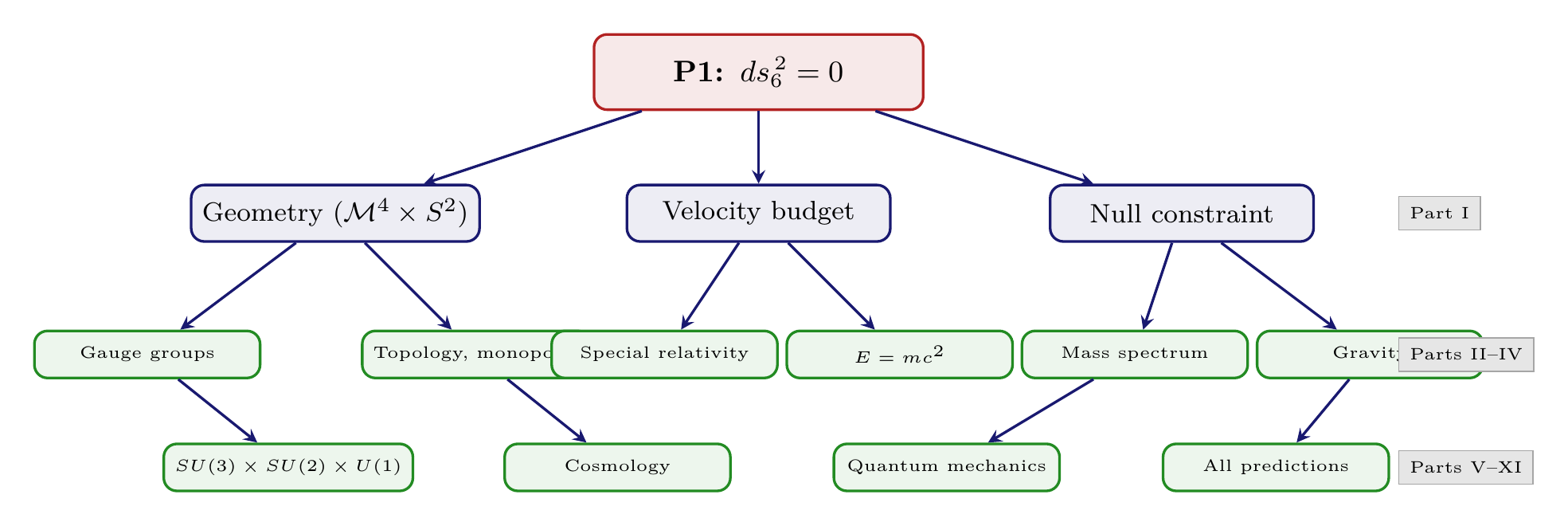
The null constraint $ds_6^{\,2} = 0$ contains, in compressed form, the seeds of all known physics. Each consequence emerges through mathematical derivation in subsequent chapters:

Table 2.3: What P1 contains and where each consequence is derived

Consequence	How It Emerges	Derived In
Special relativity	Velocity budget $v^2 + v_T^2 = c^2$	Chapter 5
$E = mc^2$	Mass IS temporal momentum	Chapter 5
$E^2 = (pc)^2 + (mc^2)^2$	6D null cone $\to$ 4D mass shell	Chapter 4
$D = 6$ uniqueness	Non-abelian gauge + monopoles	Chapter 3
Product structure $\mathcal{M}^4 \times S^2$	Null constraint forces decomposition	\Ssec:ch2-product-structure; Chapter 4
Gauge groups $SU(3) \times SU(2) \times U(1)$	$S^2$ isometry + topology	Chapters 15–19
Gravity as interface response	Tracelessness of $T^{AB}$	Chapters 6–7
Particle masses	Quantized temporal momentum	Chapters 36–42
Cosmological parameters	UV-IR balance from modulus	Part IX
Quantum mechanics	$S^2$ geometry	Part IX

The derivation chain from P1 to each of these results is presented in full, step by step, in the chapters indicated. Each link in the chain is derived explicitly with no additional postulates, no free parameters, and no fitting to data — as demonstrated in the relevant chapter. The reader is invited to verify each step independently. Figure fig:ch2-p1-fanout illustrates this branching structure.

**Figure 2.5:** Fan-out structure from P1 to all of physics. The single postulate $ds_6^{\,2} = 0$ (red) branches through geometric consequences (blue) to specific physical predictions (green). Every result in Parts I–XI traces back to this single equation. No additional postulates, free parameters, or data inputs are needed at any stage.

Having established what P1 says — the velocity budget, mass as temporal momentum, and the requirement of motion — we now address what P1 does not say. This distinction is crucial: the predictive power of TMT comes precisely from the absence of hidden assumptions.

What P1 Does NOT Say

It is equally important to state what P1 does not assume, because the absence of hidden assumptions is what gives TMT its predictive power.

P1 Does Not Assume the Topology

P1 says $ds_6^{\,2} = 0$ but does not specify what the internal manifold looks like. The fact that $K^2 = S^2$ (and not a torus, higher-genus surface, or anything else) is derived from P1 plus the requirements of stability, non-abelian gauge symmetry, and topological charge quantization. This derivation is presented in Chapter 3.

P1 Does Not Assume the Scale

P1 contains no length scale. The characteristic scale $L_\mu \approx 81\,\mu\text{m}$ emerges from the dynamical stabilization of the modulus field — the balance between UV (Planck-scale quantum gravity) and IR (cosmological horizon) effects. This derivation appears in Chapter 13.

P1 Does Not Assume Gravity

P1 says nothing about gravity. The principle that gravity couples to temporal momentum density $\rho_T = p_T/V$ (labeled P3 in the TMT organizational hierarchy: “gravity is the interface response to temporal momentum density”) is not an independent postulate but is derived from the tracelessness of the 6D energy-momentum tensor $T^{AB}$ under P1. This derivation is the content of Chapter 6.

P1 Does Not Assume Any Standard Model Parameters

The parameters of the Standard Model — the 19 of the minimal SM (3 gauge couplings, 6 quark masses, 3 charged lepton masses, 2 Higgs parameters, 4 CKM mixing parameters, and the strong CP phase) plus the neutrino sector parameters (3 neutrino masses, 3 PMNS mixing angles, 1 Dirac CP phase, and potentially 2 Majorana phases) — are all derived quantities in TMT. P1 contains zero free parameters. The derivation chain is:

$$ \text{P1 (zero parameters)} \xrightarrow{\text{derivation}} \text{SM (19 parameters derived)} $$ (2.38)

In words: The Standard Model has 19 or more free parameters that must be measured experimentally — they cannot be calculated from within the SM itself. TMT has zero free parameters. Every one of those 19+ numbers is derived from $ds_6^{\,2} = 0$ through explicit mathematical derivation. This is the central claim of this book, and the derivations fill Parts I through XI.

P1 Does Not Assume Quantum Mechanics

The postulate $ds_6^{\,2} = 0$ is a classical geometric statement. Quantum mechanics — including the Born rule, superposition, entanglement, and decoherence — emerges from the $S^2$ geometry. This emergence is derived in Part IX.

Summary: What Is and Is Not Postulated

Table 2.4: What P1 does and does not assume

POSTULATED (P1)	DERIVED (from P1)
$ds_6^{\,2} = 0$ for massive particles	$K^2 = S^2$ topology
(nothing else)	Product structure $\mathcal{M}^4 \times S^2$
	$D = 6$ uniqueness
	$L_\mu \approx 81\,\mu\text{m}$
	Gravity couples to $p_T$ density
	$SU(3) \times SU(2) \times U(1)$ gauge group
	All particle masses
	All coupling constants
	Cosmological parameters ($H_0$, $\Lambda$)
	Quantum mechanics
	Three generations
	CKM/PMNS matrices

We have seen what P1 does and does not assume. To appreciate the significance of this economy, it helps to compare TMT with the other theoretical frameworks that attempt to unify physics. The contrast is sharp.

Comparison: Postulates vs Derived Results

Postulate Count Comparison

The most striking feature of TMT is its postulate economy. Every other framework in theoretical physics requires multiple independent axioms:

Table 2.5: Postulate comparison across theoretical frameworks

Framework	Core Postulates	Free Parameters	Predictive Status
Standard Model	6 axioms$^\dagger$	19+	Works; parameters unexplained
Kaluza-Klein	Metric + topology	$\geq 2$	Gives $U(1)$ only; $g^2$ wrong by $10^{30}$
String Theory	Strings + SUSY	$10^{500}+$ landscape	No unique prediction
TMT	$\boldsymbol{ds_6^{\,2} = 0}$ only	0	SM derived (Parts I–XI); zero free parameters

Why TMT Is Not Kaluza-Klein

TMT superficially resembles traditional Kaluza-Klein theory because both use higher-dimensional mathematics. But the theories are fundamentally different in interpretation and predictive power:

Table 2.6: TMT vs. traditional extra-dimension theories

Aspect	Kaluza-Klein / String Theory	TMT
Extra dimensions	Literal hidden space	Projection structure ($S^2$)
Why invisible?	“Compactified at small scales”	Not hidden — visible as gauge forces
Gauge coupling	Volume integral $\to$ wrong by $10^{30}$	Interface overlap $\to$ correct
Uniqueness	Landscape of solutions	Single solution from $ds_6^{\,2} = 0$
Topology	Assumed (Calabi-Yau, etc.)	Derived ($S^2$ uniquely)
Predictions	None unique	Masses, couplings, cosmology

The THROUGH/AROUND distinction — why TMT is not KK

The structural reason TMT differs from Kaluza-Klein theory is the THROUGH/AROUND decomposition of the $S^2$ scaffold. In TMT, the two internal directions serve fundamentally different physical roles:

The THROUGH direction ($u = \cos\theta$, polar field) is associated with mass, the modulus, and gravity. It is the direction in which mass eigenvalues are separated and the gravitational coupling emerges.
The AROUND direction ($\phi$, azimuthal) is associated with gauge winding and charge. The $U(1)$ gauge field arises from isometry along $\phi$, and the non-abelian extension to $SU(2)$ uses the full $SO(3)$ isometry of $S^2$.

In standard Kaluza-Klein theory, this split does not exist: all internal directions contribute symmetrically through volume integration, which is precisely why the gauge coupling comes out wrong by 30 orders of magnitude. TMT's THROUGH/AROUND split ensures that gauge fields couple through interface overlap integrals (concentrated on the sphere's structure), not through volume dilution. The full development of this distinction occupies Part II (Chapters 8–14) and Part III (Chapters 15–22).

The critical distinction is the gauge coupling. Standard Kaluza-Klein theory computes gauge couplings from the volume of the internal space. The 6D-to-4D dimensional reduction relates the Planck mass to the 6D fundamental scale $M_6$ via $M_{\text{Pl}}^2 = \text{Vol}(K^2) \cdot M_6^4$. For $K^2 = S^2$ with radius $R$: $\text{Vol}(S^2) = 4\pi R^2$, giving $M_6^4 = M_{\text{Pl}}^2/(4\pi R^2)$. The 4D gauge coupling in KK theory scales as:

$$ g^2_{\text{KK}} \sim \left(\frac{M_6}{M_{\text{Pl}}}\right)^2 \sim \frac{1}{M_{\text{Pl}} \cdot R} $$ (2.39)

For any compactification radius $R$ compatible with current gravitational tests ($R \lesssim 50\,\mu\text{m}$), this coupling is catastrophically small. Taking $R \sim 10\,\mu\text{m}$ gives $M_6 \sim 10^{4}\,\text{GeV}$ and $g^2_{\text{KK}} \sim (10^4/10^{19})^2 \sim 10^{-30}$, compared to the observed gauge couplings $g^2 \sim \mathcal{O}(0.1\text{--}1)$. If $R \sim \ell_P$, one recovers $g^2 \sim 1$, but then the internal space is at the Planck scale — untestable and unable to produce TMT phenomenology. This is the gauge disaster: standard KK theory cannot simultaneously produce order-unity gauge couplings and an experimentally accessible compactification scale. The discrepancy arises because KK distributes gauge field strength over the entire compact volume, diluting it catastrophically (the precise relation $g^2_{4D} = g^2_{6D}/\text{Vol}(K^2)$ and its derivation appear in Chapter 12). TMT resolves this through the monopole topology ($\pi_2(S^2) = \mathbb{Z}$), which confines gauge fields to the $S^2$ interface and yields the correct coupling through field-space overlap integrals of monopole harmonics on $S^2$ (Chapter 20):

$$ g^2_{\text{TMT}} = \frac{4}{3\pi} \approx 0.424 $$ (2.40)

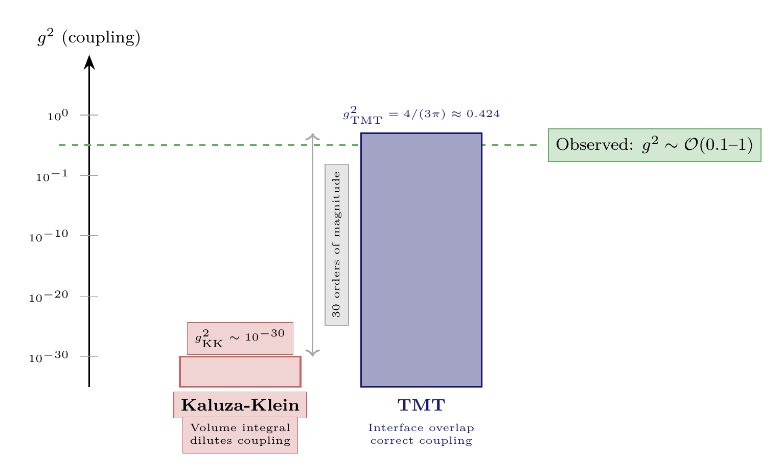
In words: The TMT gauge coupling is a ratio of three purely geometric quantities: 4 source modes from the Higgs doublet, divided by 3 gauge channels from the $SO(3)$ isometry group of $S^2$, divided by $\pi$ from the geometric spreading of monopole harmonics on the sphere. No free parameters enter. The result is order unity — matching the observed scale of gauge interactions — in stark contrast to the Kaluza-Klein prediction of $10^{-30}$.

Physical Picture: Volume Integral vs Interface Overlap: Painting a Wall vs Painting a Door Frame

The difference between KK and TMT couplings is like the difference between painting an entire wall versus painting just the door frame. In Kaluza-Klein theory, the gauge field's strength is spread uniformly over the entire volume of the compact space — like paint diluted to cover a vast wall. The result is catastrophically thin coverage (coupling $\sim 10^{-30}$). In TMT, the gauge field is concentrated at the interface between $\mathcal{M}^4$ and $S^2$ through the monopole topology ($\pi_2(S^2) = \mathbb{Z}$) — like paint applied only to the door frame where it matters. The field does not spread over the whole volume; it is confined to where the 4D and $S^2$ structures meet. The overlap integral of monopole harmonics on this interface gives a coupling of order unity: $g^2 = 4/(3\pi) \approx 0.424$. The 30-order-of-magnitude gap between KK and TMT predictions is the difference between volume dilution and interface concentration.

Why Not: Why Not Treat $S^2$ as Real Extra Dimensions?

If the $S^2$ were a literal physical space — two tiny curled-up dimensions, as in traditional Kaluza-Klein or string compactification — then gravitational experiments at short distances would reveal deviations from Newton's law. The Washington torsion-balance experiments have tested gravity down to $52\,\mu\text{m}$, within the range of the TMT scale $L_\mu \approx 81\,\mu\text{m}$. No deviations were found. If $S^2$ were real space, this would be a problem. But in TMT, $S^2$ is not physical space — it is projection structure encoding the conservation law. Gravitational experiments do not detect “extra dimensions” because there are none. The $L_\mu$ scale enters through the mass and coupling derivations, not through gravitational modifications. The scaffolding interpretation is not a philosophical preference — it is empirically required.

where $4 = n_H$ is the number of Higgs doublet degrees of freedom, $3 = n_g = \dim(SO(3))$ is the number of gauge channels from the $S^2$ isometry group, and $\pi$ is the geometric spreading factor from the monopole harmonic self-overlap integral $\int_{S^2} |Y_{q,l,m}|^4 \, d\Omega = 1/\pi$. The coupling has the structure $g^2 = \text{(source modes)} / [\text{(carrier channels)} \times \text{(spreading factor)}]$, computed from interface overlap integrals rather than volume integrals. The precise identification of this coupling with a specific Standard Model coupling constant at a specific renormalization scale, including running effects, is derived in Chapters 20–21. The key point for this chapter is that the TMT coupling is order unity — matching the observed scale of gauge interactions — whereas the standard Kaluza-Klein prediction is 30 orders of magnitude too small. This dramatic difference is depicted in Figure fig:ch2-kk-vs-tmt-coupling.

**Figure 2.6:** The gauge coupling disaster in standard Kaluza-Klein theory (red) versus TMT (blue). KK theory predicts $g^2 \sim 10^{-30}$ because it distributes gauge field strength over the full internal volume, diluting it catastrophically. TMT predicts $g^2 = 4/(3\pi) \approx 0.424$ through interface overlap integrals of monopole harmonics, matching the observed scale of gauge interactions (green dashed line). (Eqs. eq:ch2-kk-coupling–eq:ch2-tmt-coupling)

Why TMT Is Not String Theory

String theory and TMT both go beyond four dimensions, but the philosophies are opposite:

String theory starts with extended objects (strings) in 10 or 11 dimensions and derives 4D physics through compactification on a Calabi-Yau manifold. The landscape of $\sim 10^{500}$ possible compactifications means no unique prediction for low-energy physics. Supersymmetry is required but has not been observed at the LHC.

TMT starts with a single conservation law ($ds_6^{\,2} = 0$) in a unique six-dimensional framework. The topology ($S^2$), gauge groups, coupling constants, and mass spectrum are all uniquely determined. There is no landscape, no SUSY requirement, and no free parameters.

The comparison with other frameworks shows TMT's structural advantages. We now ask a deeper question: what kind of statement is P1? Understanding its philosophical status clarifies both its power and its limitations.

The Philosophical Status of P1

P1 as a Conservation Law

The deepest way to understand P1 is as a conservation law. The null constraint $ds_6^{\,2} = 0$ states that the total “velocity” through the conservation structure is always $c$. Nothing is created or destroyed — only redistributed between spatial motion and temporal motion.

This interpretation transforms what looks like an exotic geometric postulate into something physically natural: the universe conserves total velocity.

Table 2.7: TMT foundational principles and their implementation

TMT Principle	Implementation in the Theory
“6D mathematics is scaffolding”	$ds_6^{\,2} = 0$ is a conservation law, not a trajectory
“$S^2$ is projection structure”	The internal $S^2$ encodes gauge forces and mass structure, not literal hidden space
“Tesseract framework”	Energy-momentum is balanced against temporal momentum (see Core Principles \S19)
“Mass IS temporal momentum”	$p_T = mc/\gamma$ is not motion “in” a hidden space
“Gravity connects dimensions”	Gravity is the interface response mechanism

The Falsifiability of P1

A postulate in physics is only meaningful if it can, in principle, be wrong. P1 is eminently falsifiable:

(1) Direct falsification: P1 predicts specific numerical values for particle masses, coupling constants, and cosmological parameters. If any derived prediction contradicts observation beyond theoretical uncertainty, P1 is falsified.

(2) Structural falsification: P1 predicts that $D = 6$ is unique (Chapter 3). Discovery of phenomena requiring a different dimensionality would falsify P1.

(3) Gauge structure falsification: P1 predicts the Standard Model gauge group $SU(3) \times SU(2) \times U(1)$ exactly. Discovery of additional gauge bosons not predicted by this structure would falsify P1.

(4) Gravitational falsification: P1 predicts a specific form for the modified gravitational potential at short distances (Chapter 7). The Washington torsion-balance experiment has tested gravity down to $52\,\mu\text{m}$ — within the range where TMT effects would appear if 6D were literal. The null result is consistent with the scaffolding interpretation: the 6D mathematics is not physical, so the Yukawa modification does not appear in gravitational experiments. The $L_\mu = 81\,\mu\text{m}$ geometric relationship is instead confirmed through TMT's successful derivations of masses, couplings, and cosmological parameters (Parts III–IX).

The Aesthetic of P1

P1 has a simplicity that is unusual in theoretical physics. Most unification attempts add structure: extra symmetries (SUSY), extra objects (strings), extra fields (technicolor). TMT subtracts structure, arriving at a single equation that contains everything.

This is not merely aesthetic preference. Occam's razor in physics has a quantitative formulation: a theory with fewer free parameters that makes more predictions is, by Bayesian analysis, more probable. TMT has zero free parameters and makes predictions for all Standard Model parameters (the 19 of the minimal SM plus the neutrino sector) and cosmological observables. To the authors' knowledge, no other framework in the current literature achieves this scope from a single postulate.

P1 is falsifiable, aesthetic, and interpretable as a conservation law. But is it unique? Could some other geometric constraint work equally well? We now show that the answer is no: P1 is the only viable choice.

Why This Postulate and Not Another

The Uniqueness Argument

One might ask: why $ds_6^{\,2} = 0$? Why not some other geometric constraint? The answer comes from working backward from what we observe:

Step 1: We observe two empirical facts about massive particles: rest energy $E = mc^2$ and time dilation $d\tau/dt = 1/\gamma = \sqrt{1 - v^2/c^2}$. These two facts together are mathematically equivalent to a velocity budget $v^2 + v_T^2 = c^2$ once we identify $v_T \equiv c/\gamma$ — the quantity whose physical content is the time-dilation factor, and whose rest-frame value ($v_T = c$) gives $E = mc^2$ through $p_T = mv_T = mc$.

Step 2: The velocity budget is mathematically equivalent to a null constraint in a higher-dimensional framework: $ds_6^{\,2} = 0$ on $\mathcal{M}^4 \times K^2$.

Step 3: For the constraint to produce non-abelian gauge symmetry and topological charge quantization (both observed), $K^2$ must be $S^2$ and $D$ must be 6 (Chapter 3).

Step 4: The null constraint is the simplest such condition. Alternatives — timelike constraints ($ds_6^{\,2} < 0$), spacelike constraints ($ds_6^{\,2} > 0$), or more complex algebraic conditions — either fail to reproduce observed physics or reduce to the null case in the appropriate limit.

What If P1 Were Different?

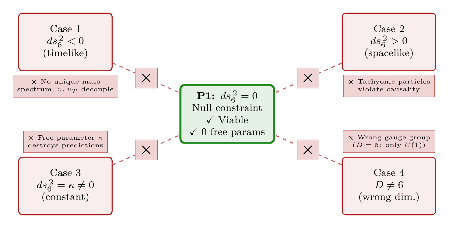
Theorem 2.3 (Counterfactual Analysis of P1)

If P1 were replaced by any of the following alternatives, the resulting theory would fail to reproduce observed physics:

$ds_6^{\,2} < 0$ (timelike in 6D): No velocity budget; $v$ and $v_T$ decouple
$ds_6^{\,2} > 0$ (spacelike in 6D): Tachyonic; violates causality
$ds_6^{\,2} = \kappa \neq 0$ (constant): Adds a free parameter; loses predictive power
$ds_D^2 = 0$ with $D \neq 6$: Wrong gauge structure (Chapter 3)

Proof.

Derivation Roadmap

Proof roadmap (4 cases to eliminate):

Timelike ($ds_6^{\,2} < 0$): velocity budget becomes an inequality, destroying the unique mass spectrum
Spacelike ($ds_6^{\,2} > 0$): forces tachyonic modes (imaginary mass), violating causality
Non-zero constant ($ds_6^{\,2} = \kappa \neq 0$): introduces a free parameter, destroying predictive power
Wrong dimension ($D \neq 6$): produces the wrong gauge group (too small or too large)

Each case is independent — eliminating all four establishes that P1 is the unique viable choice.

Case 1 ($ds_6^{\,2} < 0$): If the 6D interval is timelike, then $ds_4^2 + ds_{S^2}^2 < 0$. The inequality (rather than equality) means the $S^2$ projection contribution $ds_{S^2}^2$ is not uniquely determined by the 4D interval $ds_4^2$. Specifically, the constraint allows any $ds_{S^2}^2$ in the range $[0, |ds_4^2|)$:

If $ds_{S^2}^2 = 0$: the $S^2$ contribution is absent entirely, and temporal momentum vanishes. The particle has no mass-temporal momentum coupling.
If $0 < ds_{S^2}^2 < |ds_4^2|$: the $S^2$ contribution is nonzero but does not fully compensate the 4D interval. Temporal momentum exists but is not uniquely fixed — it can take any value in a continuous range for a given 4D motion.

In both subcases, the velocity budget $v^2 + v_T^2 = c^2$ is replaced by the inequality $v^2 + v_T^2 < c^2$, which does not uniquely determine $v_T$ from $v$. The one-to-one mapping between mass and temporal momentum eigenvalue — which is what makes the mass spectrum discrete and predictable in TMT — is destroyed. No unique mass spectrum can be derived from a timelike constraint.

Case 2 ($ds_6^{\,2} > 0$): If the 6D interval is spacelike, then $ds_4^2 + ds_{S^2}^2 > 0$. In momentum space: $g_{\mu\nu}k^\mu k^\nu + h_{ij}k^ik^j > 0$. Since $h_{ij}k^ik^j > 0$ (positive-definite metric on $S^2$), this requires $g_{\mu\nu}k^\mu k^\nu > -h_{ij}k^ik^j + \epsilon$ for some $\epsilon > 0$. The 4D mass-shell identification $g_{\mu\nu}k^\mu k^\nu = -m^2c^2$ then gives $-m^2c^2 > -h_{ij}k^ik^j + \epsilon$, i.e., $m^2c^2 < h_{ij}k^ik^j - \epsilon$. For sufficiently small $K^2$ eigenvalues, this forces $m^2 < 0$ — the particles are tachyonic (imaginary mass in 4D). Tachyonic particles propagate superluminally and violate causality, contradicting observation. No consistent quantum field theory with tachyonic fundamental excitations reproduces observed physics.

Checkpoint (Cases 1–2 of 4): We have eliminated the timelike case (no unique mass spectrum) and the spacelike case (tachyonic particles). The remaining two cases consider alternative values and dimensionalities.

Case 3 ($ds_6^{\,2} = \kappa \neq 0$): A non-zero constant means $ds_4^2 + ds_{S^2}^2 = \kappa$ (where $\kappa$ is a fixed constant with dimensions of length$^2$ in coordinate space; we use $\kappa$ rather than $k^2$ to avoid confusion with the six-momentum $k^A$). Passing to the mass-shell relation (absorbing dimensional factors from the coordinate-to-momentum mapping into $\kappa$, so that $\kappa$ now carries dimensions of momentum$^2$), this gives $g_{\mu\nu}k^\mu k^\nu + h_{ij}k^ik^j = \kappa$, so the 4D mass-shell relation becomes:

$$ -m^2 c^2 + h_{ij}k^ik^j = \kappa \quad \Longrightarrow \quad m^2 c^2 = h_{ij}k^ik^j - \kappa $$ (2.41)

This has three fatal consequences. First, if $\kappa > 0$ (spacelike), then $m^2 c^2 = h_{ij}k^ik^j - \kappa < h_{ij}k^ik^j$, and for sufficiently small $K^2$ eigenvalues, $m^2 < 0$ (tachyonic modes appear), reducing to the pathology of Case 2. Second, if $\kappa < 0$ (timelike), then $m^2 c^2 = h_{ij}k^ik^j + |\kappa|$: every mass eigenvalue is shifted upward by $|\kappa|$. The spectrum remains discrete, but every predicted mass now depends on the arbitrary constant $|\kappa|$ — a free parameter with no physical origin that must be tuned to reproduce observed masses, reinforcing the third objection below. Third, for any $\kappa \neq 0$, the constant introduces a free parameter with no physical origin, converting TMT from a zero-parameter theory into a one-parameter fitting exercise. Every derived quantity (masses, couplings, cosmological parameters) would depend on $\kappa$, destroying predictive power. There is no natural limit $\kappa \to 0$ that recovers the null case without fine-tuning, since $\kappa$ appears additively in all mass predictions.

Case 4 ($D \neq 6$): This is analyzed in detail in Chapter 3 (the Dimension Theorem). $D = 5$ gives only $U(1)$ gauge symmetry (cannot produce $W^\pm$, $Z^0$); $D = 7$ gives $SO(4)$ which is too large and has $\pi_2(S^3) = 0$ (no monopoles); $D \geq 8$ gives excessively large gauge groups requiring fine-tuned symmetry breaking. Only $D = 6$ with $K^2 = S^2$ gives the observed Standard Model structure with topological charge quantization.

Each alternative either fails phenomenologically, introduces free parameters, or violates fundamental physics (causality, unitarity). P1 as stated is the unique constraint producing a viable, parameter-free theory. □

(See: Chapter 2, \Ssec:ch2-uniqueness-argument, \Ssec:ch2-falsifiability) □

Summary: The counterfactual analysis eliminates every alternative to P1. Timelike constraints decouple the velocity budget and destroy the discrete mass spectrum. Spacelike constraints produce tachyons. Non-zero constants introduce free parameters. Wrong dimensionality gives wrong gauge groups. The null constraint $ds_6^{\,2} = 0$ in six dimensions is the unique choice producing a viable, parameter-free theory. The four alternatives and their failure modes are summarized in Figure fig:ch2-counterfactual-analysis.

**Figure 2.7:** Counterfactual analysis of P1 (Theorem thm:P1-Ch2-counterfactual). Four alternative constraints are tested and eliminated: timelike (no unique mass spectrum), spacelike (tachyonic), constant nonzero (free parameter), and wrong dimensionality (wrong gauge group). Only the null constraint $ds_6^{\,2} = 0$ produces a viable, parameter-free theory matching observation.

P1 and the Arrow of Explanation

The arrow of explanation in TMT runs:

$$ \text{P1} \to \text{geometry} \to \text{gauge forces} \to \text{particle physics} \to \text{cosmology} $$ (2.42)

In words: The arrow of explanation runs forward from postulate to prediction, never backward from observation to fitting. P1 determines the geometry; the geometry determines the gauge forces; the gauge forces determine particle physics; and particle physics determines cosmology. At no stage does an observed number enter as input. This is what makes TMT a derivation framework rather than a fitting framework.

Physical Picture: The Arrow of Explanation: A River, Not a Lake

Most theories in physics are like lakes: they collect observed parameters from experiment and hold them as standing water, with no explanation of where the water came from. The Standard Model, for instance, has 19+ measured parameters sitting in its lagrangian, each put there by hand. TMT is like a river: it starts from a single spring (P1: $ds_6^{\,2} = 0$) and flows downhill through geometry, gauge structure, particle physics, and cosmology. Each prediction is downstream of the postulate. The river never flows backward — no experimental measurement is pumped upstream to serve as input. If any downstream prediction contradicts experiment, the spring itself is wrong, and the entire river must be reconsidered. This is what makes TMT maximally falsifiable: a single failure anywhere downstream falsifies the single source.

At no point in this chain is an observation used as input (except for P1 itself, which encodes $E = mc^2$). The chain is deductive, not phenomenological. This makes TMT unique among proposals for physics beyond the Standard Model: it is a derivation framework, not a fitting framework.

We have now derived all the main results of this chapter and shown that the postulate P1 is unique. Before moving on, it is valuable to see the entire logical chain at a glance — from postulate to final result, with every step labeled.

Derivation Chain Summary

The logical flow of Chapter 2 is summarized in Figure fig:ch2-derivation-chain-flowchart.

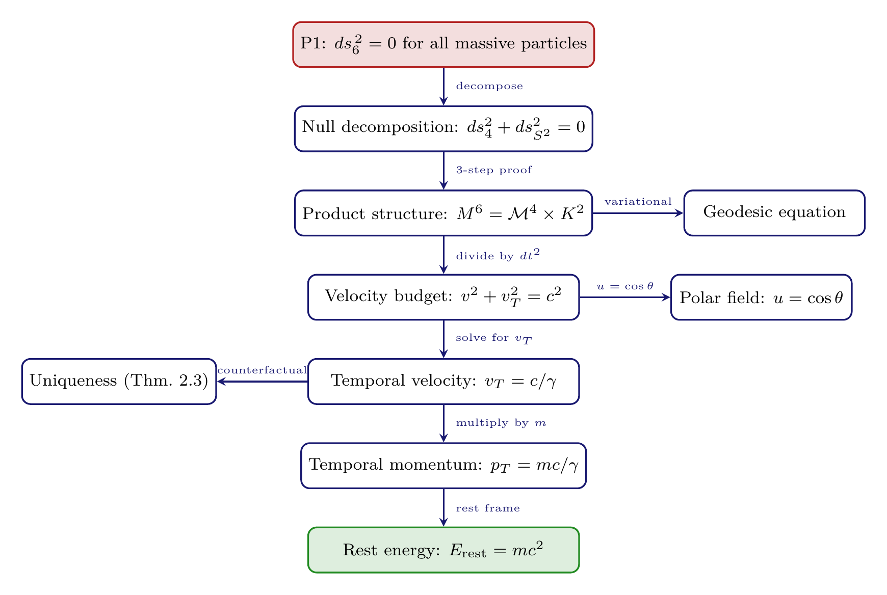
**Figure 2.8:** Derivation chain for Chapter 2. Starting from P1 (red), each result follows by a single logical step (labeled on arrows). The product structure step uses P1 together with three observational inputs (position-independent masses, 4D covariance, vacuum definition); all subsequent steps are strictly deductive from the product structure. Side branches show the geodesic equation (from product structure via variational principle), polar field representation (from the velocity budget), and uniqueness analysis (from temporal velocity).

Key Result

Derivation Chain for Chapter 2: The Single Postulate

Step	Result	Status	Source
1	P1: $ds_6^{\,2} = 0$	POSTULATE	Eq.	nbsp;eq:ch2-P1
2	Null decomposition: $ds_4^2 + ds_{S^2}^2 = 0$	PROVEN	Eq.	nbsp;eq:ch2-null-decomposition
3	Product structure: $M^6 = \mathcal{M}^4 \times K^2$ ($K^2 = S^2$ via Ch.	nbsp;3)	DERIVED	Theorem	nbsp;thm:P1-Ch2-product-structure
4	Velocity budget: $v^2 + v_T^2 = c^2$	PROVEN	Eq.	nbsp;eq:ch2-velocity-budget
5	Temporal velocity: $v_T = c/\gamma$	PROVEN	Eq.	nbsp;eq:ch2-temporal-velocity
6	Temporal momentum: $p_T = mc/\gamma$	PROVEN	Eq.	nbsp;eq:ch2-temporal-momentum-def
7	Rest energy: $E_{\text{rest}} = p_T c\big\|_{v=0} = mc^2$	PROVEN	Eq.	nbsp;eq:ch2-emc2-from-pT
8	Geodesic equation from variational principle	PROVEN	Eq.	nbsp;eq:ch2-geodesic-6d
9	Polar field representation: $u = \cos\theta$, $\sqrt{g} = R_0^2$	PROVEN	Eq.	nbsp;eq:ch2-s2-metric-polar
10	Uniqueness of P1 (counterfactual)	PROVEN	Theorem	nbsp;thm:P1-Ch2-counterfactual

Visualizations

The Velocity Budget

**Figure 2.9:** The velocity budget from P1. Every particle lies on the quarter circle $v^2 + v_T^2 = c^2$. At rest, all velocity is temporal ($v_T = c$). For photons, all velocity is spatial ($v = c$). Intermediate particles partition velocity between spatial and temporal components.

The Polar Field Representation of $S^2$

**Figure 2.10:** The polar field representation maps the $S^2$ sphere (left) to a flat rectangle $[-1,+1] \times [0,2\pi)$ (right) via $u = \cos\theta$. The “around” direction ($\phi$, green) carries gauge physics; the “through” direction ($u$, red) carries mass/gravity physics. In the polar field representation, the metric determinant $\sqrt{g} = R_0^2$ is constant — every integral over $S^2$ becomes a flat rectangular integral with no angular weight factors.

The Postulate Comparison

**Figure 2.11:** Comparison of theoretical frameworks. TMT derives what other theories assume or cannot predict, using a single postulate with zero free parameters.

The derivation chain above captures the full logical content of Chapter 2 in ten explicit steps. We now summarize the results and look ahead to Chapter 3, where the first major consequence of P1 is derived: the uniqueness of six dimensions.

Chapter Summary

This chapter has introduced the single postulate of Temporal Momentum Theory:

Proven

P1 — The Null Constraint:

$$ ds_6^{\,2} = 0 \quad \text{for all massive particles} $$

Physical content: The velocity budget $v^2 + v_T^2 = c^2$ — every particle partitions the universal speed $c$ between spatial velocity and temporal velocity. Mass is temporal momentum: $p_T = mc/\gamma$.

What P1 contains: The seeds of all known physics — the Standard Model and cosmology — in compressed form (derived in Parts I–XI).

What P1 assumes: Nothing beyond itself. Zero free parameters.

What would falsify P1: Any derived prediction contradicting observation.

The remainder of this book derives the consequences of P1, one theorem at a time, building the complete structure of known physics from this single geometric constraint. The next chapter (Chapter 3) derives the first major consequence: that $D = 6$ is the unique dimensionality consistent with observed gauge symmetry and topological charge quantization.

Verification Code

The mathematical derivations and proofs in this chapter can be independently verified using the formal and computational scripts below.

◆ Lean 4 Formal proof verification Coming Soon ● Python Numerical verification & plots Coming Soon ★ Mathematica Symbolic computation & CAS verification Coming Soon

All verification code is open source. See the complete verification index for all chapters.

Index Type	Labels	Range	Space
Capital Latin	\(A, B, C, \ldots\)	\(0, 1, 2, 3, 5, 6\)	Full 6D scaffolding
Greek	\(\mu, \nu, \rho, \ldots\)	\(0, 1, 2, 3\)	4D spacetime \(\mathcal{M}^4\)
Lowercase Latin (spatial)	\(i, j, k, \ldots\)	\(1, 2, 3\)	3D spatial (in purely 4D context)
Lowercase Latin (\(S^2\))	\(i, j\) or \(a, b\)	\(5, 6\)	\(S^2\) projection (in 6D decomposition context)

The Single Postulate

Statement of P1: \(ds_6^{\,2} = 0\)

What the Postulate Asserts

The Vocabulary of P1

Mathematical Form of the Null Geodesic Hypothesis

The Null Constraint in Momentum Space

The Product Structure

The 6D Metric

The Polar Field Representation

The Geodesic Equation

Index Conventions

What P1 Says: Massive Particles Are Null in 6D

The Core Physical Content

What P1 Unifies

What P1 Does NOT Say

P1 Does Not Assume the Topology

P1 Does Not Assume the Scale

P1 Does Not Assume Gravity

P1 Does Not Assume Any Standard Model Parameters

P1 Does Not Assume Quantum Mechanics

Summary: What Is and Is Not Postulated

Comparison: Postulates vs Derived Results

Postulate Count Comparison

Why TMT Is Not Kaluza-Klein

Why TMT Is Not String Theory

The Philosophical Status of P1

P1 as a Conservation Law

The Falsifiability of P1

The Aesthetic of P1

Why This Postulate and Not Another

The Uniqueness Argument

What If P1 Were Different?

P1 and the Arrow of Explanation

Derivation Chain Summary

Visualizations

The Velocity Budget

The Polar Field Representation of \(S^2\)

The Postulate Comparison

Chapter Summary

Verification Code

Term	Precise Meaning
“Conservation structure”	The mathematical framework encoding how energy, momentum, and mass interrelate. Not a literal space.
“\(ds_6^{\,2}\)”	The line element in the six-dimensional scaffolding framework \(\mathcal{M}^4 \times S^2\).
“Null constraint”	The condition \(ds_6^{\,2} = 0\), stating that the 4D and \(S^2\) contributions exactly cancel.
“Massive particles”	All particles with rest mass \(m > 0\): electrons, quarks, neutrinos, \(W\), \(Z\), Higgs.
“Scaffolding”	The 6D mathematics is a computational tool, not a claim about the number of spatial dimensions.
“Velocity budget”	The constraint \(v^2 + v_T^2 = c^2\): every particle partitions the universal speed \(c\) between spatial velocity \(v\) and temporal velocity \(v_T\).
“Temporal momentum”	The momentum associated with temporal velocity: \(p_T = mv_T = mc/\gamma\). Equal to \(mc\) at rest; vanishes for photons.

Consequence	How It Emerges	Derived In
Special relativity	Velocity budget \(v^2 + v_T^2 = c^2\)	Chapter 5
\(E = mc^2\)	Mass IS temporal momentum	Chapter 5
\(E^2 = (pc)^2 + (mc^2)^2\)	6D null cone \(\to\) 4D mass shell	Chapter 4
\(D = 6\) uniqueness	Non-abelian gauge + monopoles	Chapter 3
Product structure \(\mathcal{M}^4 \times S^2\)	Null constraint forces decomposition	\Ssec:ch2-product-structure; Chapter 4
Gauge groups \(SU(3) \times SU(2) \times U(1)\)	\(S^2\) isometry + topology	Chapters 15–19
Gravity as interface response	Tracelessness of \(T^{AB}\)	Chapters 6–7
Particle masses	Quantized temporal momentum	Chapters 36–42
Cosmological parameters	UV-IR balance from modulus	Part IX
Quantum mechanics	\(S^2\) geometry	Part IX

POSTULATED (P1)	DERIVED (from P1)
\(ds_6^{\,2} = 0\) for massive particles	\(K^2 = S^2\) topology
(nothing else)	Product structure \(\mathcal{M}^4 \times S^2\)
	\(D = 6\) uniqueness
	\(L_\mu \approx 81\,\mu\text{m}\)
	Gravity couples to \(p_T\) density
	\(SU(3) \times SU(2) \times U(1)\) gauge group
	All particle masses
	All coupling constants
	Cosmological parameters (\(H_0\), \(\Lambda\))
	Quantum mechanics
	Three generations
	CKM/PMNS matrices

Framework	Core Postulates	Free Parameters	Predictive Status
Standard Model	6 axioms\(^\dagger\)	19+	Works; parameters unexplained
Kaluza-Klein	Metric + topology	\(\geq 2\)	Gives \(U(1)\) only; \(g^2\) wrong by \(10^{30}\)
String Theory	Strings + SUSY	\(10^{500}+\) landscape	No unique prediction
TMT	\(\boldsymbol{ds_6^{\,2} = 0}\) only	0	SM derived (Parts I–XI); zero free parameters

Aspect	Kaluza-Klein / String Theory	TMT
Extra dimensions	Literal hidden space	Projection structure (\(S^2\))
Why invisible?	“Compactified at small scales”	Not hidden — visible as gauge forces
Gauge coupling	Volume integral \(\to\) wrong by \(10^{30}\)	Interface overlap \(\to\) correct
Uniqueness	Landscape of solutions	Single solution from \(ds_6^{\,2} = 0\)
Topology	Assumed (Calabi-Yau, etc.)	Derived (\(S^2\) uniquely)
Predictions	None unique	Masses, couplings, cosmology

TMT Principle	Implementation in the Theory
“6D mathematics is scaffolding”	\(ds_6^{\,2} = 0\) is a conservation law, not a trajectory
“\(S^2\) is projection structure”	The internal \(S^2\) encodes gauge forces and mass structure, not literal hidden space
“Tesseract framework”	Energy-momentum is balanced against temporal momentum (see Core Principles \S19)
“Mass IS temporal momentum”	\(p_T = mc/\gamma\) is not motion “in” a hidden space
“Gravity connects dimensions”	Gravity is the interface response mechanism

Step	Result	Status	Source
1	P1: \(ds_6^{\,2} = 0\)	POSTULATE	Eq.	nbsp;eq:ch2-P1
2	Null decomposition: \(ds_4^2 + ds_{S^2}^2 = 0\)	PROVEN	Eq.	nbsp;eq:ch2-null-decomposition
3	Product structure: \(M^6 = \mathcal{M}^4 \times K^2\) (\(K^2 = S^2\) via Ch.	nbsp;3)	DERIVED	Theorem	nbsp;thm:P1-Ch2-product-structure
4	Velocity budget: \(v^2 + v_T^2 = c^2\)	PROVEN	Eq.	nbsp;eq:ch2-velocity-budget
5	Temporal velocity: \(v_T = c/\gamma\)	PROVEN	Eq.	nbsp;eq:ch2-temporal-velocity
6	Temporal momentum: \(p_T = mc/\gamma\)	PROVEN	Eq.	nbsp;eq:ch2-temporal-momentum-def
7	Rest energy: \(E_{\text{rest}} = p_T c\big\|_{v=0} = mc^2\)	PROVEN	Eq.	nbsp;eq:ch2-emc2-from-pT
8	Geodesic equation from variational principle	PROVEN	Eq.	nbsp;eq:ch2-geodesic-6d
9	Polar field representation: \(u = \cos\theta\), \(\sqrt{g} = R_0^2\)	PROVEN	Eq.	nbsp;eq:ch2-s2-metric-polar
10	Uniqueness of P1 (counterfactual)	PROVEN	Theorem	nbsp;thm:P1-Ch2-counterfactual