
Spherical Harmonics
This appendix provides the complete mathematical framework for spherical harmonics on \(S^2\) — the mathematical scaffolding on which the projection interface structure is built in TMT. We cover ordinary spherical harmonics, monopole harmonics, completeness relations, coupling formulas, and the numerical values essential to TMT calculations.
Ordinary Spherical Harmonics
Definition and Orthonormality
The ordinary spherical harmonics \(Y_{\ell m}(\theta, \phi)\) form a complete orthonormal basis for square-integrable functions on the 2-sphere \(S^2\). We use the standard physics convention where \(\theta \in [0, \pi]\) is the polar angle and \(\phi \in [0, 2\pi)\) is the azimuthal angle on \(S^2\).
The ordinary spherical harmonics are defined as:
where \(\ell = 0, 1, 2, \ldots\) is the angular momentum quantum number, \(m = -\ell, -\ell+1, \ldots, \ell-1, \ell\) is the magnetic quantum number, and \(P_{\ell}^{|m|}\) denotes the associated Legendre polynomial.
Physical interpretation: In TMT, \(Y_{\ell m}\) represent the harmonic decomposition of fields on the projection interface \(S^2\). The index \(\ell\) characterizes the angular momentum structure of the projection, while \(m\) tracks the magnetic quantum number corresponding to rotations about the interface axis.
The ordinary spherical harmonics satisfy the orthonormality condition:
where the integration is over the solid angle \(d\Omega = \sin\theta \, d\theta \, d\phi\), and \(\delta\) denotes the Kronecker delta.
The orthonormality follows directly from the orthogonality properties of Legendre polynomials and the exponential basis \(e^{im\phi}\):
Step 1 — Angular (\(\phi\)) orthogonality: The exponential factors satisfy:
Step 2 — Polar (\(\theta\)) orthogonality: The associated Legendre polynomials satisfy:
Step 3 — Combining with normalization: The normalization constant in Eq. eq:Y-lm-definition is chosen precisely so that the product of the normalization factor, the Legendre integral result, and the exponential integral yields unity:
Therefore, the product of the Legendre and exponential integrals with the correct normalization yields exactly \(\delta_{\ell\ell'} \delta_{mm'}\). □
First Few Harmonics: Explicit Examples
For reference, the first few ordinary spherical harmonics in explicit form are:
Polar Field Form of Spherical Harmonics
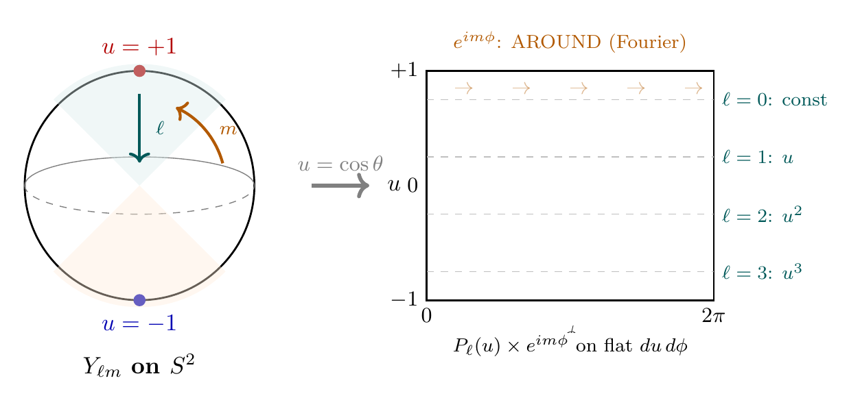
In the polar field variable \(u = \cos\theta\), all spherical harmonics become polynomials in \(u\) multiplied by Fourier modes in \(\phi\), and the integration measure becomes flat:
The general formula Eq. (eq:Y-lm-definition) becomes:
The first few harmonics in polar form:
Harmonic | Spherical form | Polar form | Polynomial degree |
|---|---|---|---|
| \(Y_{00}\) | \(1/\sqrt{4\pi}\) | \(1/\sqrt{4\pi}\) | 0 (constant) |
| \(Y_{10}\) | \(\sqrt{3/4\pi}\cos\theta\) | \(\sqrt{3/4\pi}\,u\) | 1 (linear) |
| \(Y_{20}\) | \(\sqrt{5/4\pi}(\frac{3}{2}\cos^2\!\theta{-}\frac{1}{2})\) | \(\sqrt{5/4\pi}(\frac{3}{2}u^2{-}\frac{1}{2})\) | 2 (quadratic) |
| \(Y_{\ell 0}\) | \(P_\ell(\cos\theta)\) | \(P_\ell(u)\) | \(\ell\) |
| \(Y_{\ell,\pm\ell}\) | \(\sin^\ell\!\theta\,e^{\pm i\ell\phi}\) | \((1-u^2)^{\ell/2}\,e^{\pm i\ell\phi}\) | \(\ell\) (in \(u^2\)) |
Key insight: The harmonic decomposition on \(S^2\) is literally the polynomial\(\times\)Fourier decomposition on the flat rectangle \([-1,+1]\times[0,2\pi)\). The \(u\)-dependence gives the THROUGH (mass/chirality) structure via Legendre polynomials of degree \(\ell\); the \(\phi\)-dependence gives the AROUND (gauge/charge) structure via Fourier modes \(e^{im\phi}\) of frequency \(m\).
Scaffolding note: The polar field variable \(u = \cos\theta\) is a coordinate choice, not a new physical assumption. The polynomial interpretation of spherical harmonics as functions on the flat rectangle \([-1,+1]\times[0,2\pi)\) provides computational transparency: all integrals become polynomial \(\times\) Fourier integrals with flat Lebesgue measure \(du\,d\phi\).
The Addition Theorem
A key property of spherical harmonics is the addition theorem, which expresses the dependence on relative angles in terms of a sum over harmonics.
For any two directions \(\hat{n}\) and \(\hat{n}'\) on the sphere separated by angle \(\gamma\) (where \(\cos\gamma = \hat{n} \cdot \hat{n}'\)), the addition theorem states:
where \(P_{\ell}\) is the Legendre polynomial of degree \(\ell\).
Physical interpretation in TMT: The addition theorem is crucial for computing interactions between fields on different regions of the interface \(S^2\). When evaluating coupling integrals between fields localized at different points on the sphere, the addition theorem allows decomposition in terms of harmonic modes.
Eigenvalue Problem on \(S^2\)
The ordinary spherical harmonics are the eigenfunctions of the Laplacian operator on \(S^2\).
The Laplacian on \(S^2\) (in the standard metric with radius \(R\)) acting on spherical harmonics yields:
The eigenvalues are therefore:
Each eigenvalue \(\lambda_{\ell}\) has multiplicity \(2\ell+1\), corresponding to the \(2\ell+1\) degenerate eigenfunctions \(Y_{\ell m}\) for \(m = -\ell, \ldots, \ell\).
This is a standard result in mathematical physics. The Laplacian in spherical coordinates on \(S^2\) (with \(\theta\) and \(\phi\) coordinates) is:
Substituting \(f = Y_{\ell m}(\theta, \phi)\) where \(Y_{\ell m} = P_{\ell}^{|m|}(\cos\theta) e^{im\phi}\), the \(\phi\)-derivatives act directly on the exponential:
The \(\theta\)-derivative acts on the associated Legendre polynomial via the well-known eigenvalue equation:
Rearranging and combining contributions:
(Here we have included the factor of \(1/R^2\) from the metric on a sphere of radius \(R\).)
Therefore: \(-\nabla^2 Y_{\ell m} = \frac{\ell(\ell+1)}{R^2} Y_{\ell m}\), confirming the eigenvalue result. □
Polar Form of the \(S^2\) Laplacian
In the polar variable \(u = \cos\theta\), the \(S^2\) Laplacian takes the Legendre operator form:
The eigenvalue equation \(-\nabla^2_{S^2}Y_{\ell m} = \lambda_\ell Y_{\ell m}\) separates into THROUGH and AROUND:
—
Monopole Harmonics
The Wu-Yang Monopole on \(S^2\)
The monopole harmonics \(Y_{q,\ell,m}\) are the generalization of ordinary spherical harmonics to include a magnetic monopole of charge \(q\) on \(S^2\). These are fundamental to TMT because the Higgs mechanism on the projection interface requires non-trivial U(1) bundle structure, which is mathematically encoded as a monopole.
The second homotopy group \(\pi_2(S^2)\) counts equivalence classes of maps from \(S^2\) to \(S^2\). The key result is that any map \(f: S^2 \to S^2\) can be classified by the winding number.
Step 1: By the Hurewicz theorem, \(\pi_2(S^2) \cong H_2(S^2; \mathbb{Z})\), where \(H_2\) denotes the second homology group.
Step 2: The homology of \(S^2\) is:
Step 3: Therefore \(\pi_2(S^2) = H_2(S^2; \mathbb{Z}) = \mathbb{Z}\), and each element \(n \in \mathbb{Z}\) corresponds to a distinct homotopy class.
Step 4: In physics, \(n\) is the monopole charge. The canonical generator is \(n = 1\), the minimal non-trivial monopole. □
Physical interpretation in TMT: The projection interface \(S^2\) must support a monopole of charge \(q = 1\) (the minimal non-trivial configuration) to generate the correct gauge structure for the Standard Model. This is not an assumption but a consequence of requiring non-trivial U(1) bundle structure, which is essential for charge quantization.
Wu-Yang Monopole Potential
The Wu-Yang construction describes a monopole on \(S^2\) using two overlapping coordinate patches covering the northern and southern hemispheres.
For a monopole of charge \(q\) on \(S^2\), the Wu-Yang gauge potential is defined in two patches:
Northern patch (covering \(\theta < \pi/2 + \epsilon\)):
Southern patch (covering \(\theta > \pi/2 - \epsilon\)):
On the overlap region, the two potentials are related by a gauge transformation with winding number \(2q\pi\), ensuring charge consistency.
Polar form of the Wu-Yang potential. In the polar variable \(u = \cos\theta\), the monopole connection for \(q = 1\) becomes remarkably simple:
Key properties: The Wu-Yang construction manifestly preserves rotational symmetry because the two patches transform under rotations in exactly the right way to maintain the gauge structure. There is no singularity other than the unavoidable Dirac string, which can be placed anywhere and has no physical significance.
Monopole Harmonics: Definition and Orthogonality
Monopole harmonics are eigenfunctions of the covariant Laplacian (Laplacian coupled to the monopole gauge field) on \(S^2\).
Monopole harmonics \(Y_{q,\ell,m}(\theta, \phi)\) are the eigenfunctions of the covariant Laplacian in the presence of a monopole of charge \(q\) on \(S^2\). They satisfy:
where \(\nabla^2_{\text{cov}} = \nabla^2 - i q A_{\mu} \partial^{\mu}\) is the covariant Laplacian and \(\ell\) is now constrained by \(\ell \geq |q|\).
The monopole harmonics are labeled by three quantum numbers:
- \(q\) — the monopole charge (integer)
- \(\ell\) — the angular momentum quantum number, \(\ell = |q|, |q|+1, |q|+2, \ldots\)
- \(m\) — the magnetic quantum number, \(m = -\ell, -\ell+1, \ldots, \ell-1, \ell\)
Crucial difference from ordinary harmonics: When \(q \neq 0\), the minimum value of \(\ell\) is no longer 0, but rather \(\ell = |q|\). For \(q = 1\) (the monopole charge required in TMT), the lowest harmonic has \(\ell = 1\) (no \(\ell = 0\) mode).
Monopole harmonics with the same monopole charge \(q\) satisfy orthonormality:
Monopole harmonics with different charges are orthogonal to each other:
The orthonormality of monopole harmonics follows from the same principles as for ordinary harmonics, but adapted to the covariant Laplacian. The gauge transformation property ensures that despite the monopole gauge field, the inner product remains well-defined.
Step 1: Define the inner product on \(S^2\) with the standard area measure \(d\Omega = \sin\theta \, d\theta \, d\phi\).
Step 2: The covariant derivative operator \(\nabla_{\text{cov}}\) is self-adjoint with respect to this inner product (this can be verified by integration by parts, using the fact that the monopole gauge field is real).
Step 3: Since \(\nabla^2_{\text{cov}} Y_{q,\ell,m} = -\frac{\ell(\ell+1)}{R^2} Y_{q,\ell,m}\) and \(\nabla^2_{\text{cov}} Y_{q,\ell',m'} = -\frac{\ell'(\ell'+1)}{R^2} Y_{q,\ell',m'}\), the eigenfunctions are orthogonal when they correspond to different eigenvalues.
Step 4: When \(\ell \neq \ell'\), the eigenvalues differ and orthogonality follows immediately. When \(\ell = \ell'\) but \(m \neq m'\), orthogonality follows from rotational symmetry.
Step 5: For different monopole charges \(q\) and \(q'\), the covariant Laplacians are different operators, and their eigenfunctions are orthogonal. □
Monopole Harmonics for \(q=1\): Relation to Ordinary Harmonics
For TMT, the monopole charge is \(q = 1\). In this case, monopole harmonics have an intimate connection to ordinary harmonics.
For monopole charge \(q = 1\), the monopole harmonics can be expressed in terms related to ordinary spherical harmonics with specific structural modifications. The monopole harmonics with \(\ell \geq 1\) and \(m = -\ell, \ldots, \ell\) form a complete basis orthogonal to the \(\ell = 0\) mode.
Key feature: Unlike ordinary harmonics (which include \(\ell = 0\)), monopole harmonics with \(q = 1\) have \(\ell_{\min} = 1\). The absence of the \(\ell = 0\) mode is a direct topological consequence of the monopole structure.
The monopole harmonics can be written as:
where \(f_{\ell,m}\) are specific functions (related to Jacobi polynomials) and \(\ell \geq 1\).
Physical meaning in TMT: The factor \(e^{i\phi/2}\) in Eq. eq:monopole-q1-form encodes the monopole's topological charge. A charged particle that encircles the monopole gains a phase \(e^{i\cdot 1 \cdot 2\pi/2} = e^{i\pi} = -1\), which is the distinctive signature of monopole topology. This phase is crucial for understanding charge quantization in TMT.
—
Completeness Relations on \(S^2\)
Completeness for Ordinary Harmonics
The ordinary spherical harmonics form a complete orthonormal basis for \(L^2(S^2)\), the space of square-integrable functions on \(S^2\).
For any function \(f \in L^2(S^2)\), the expansion:
converges in the \(L^2\) sense, where the coefficients are:
Moreover, the completeness relation holds:
where \(\delta(\Omega - \Omega')\) is the Dirac delta function on the sphere.
The completeness of ordinary spherical harmonics is a standard result in functional analysis and is proven using the completeness of Legendre polynomials and the Fourier basis in the azimuthal direction.
Step 1 — Fourier completeness in \(\phi\): For fixed \(\theta\), the functions \(\{e^{im\phi}\}_{m \in \mathbb{Z}}\) form a complete orthonormal basis for \(L^2([0, 2\pi])\). Therefore, any \(\phi\)-dependent function can be expanded in Fourier modes.
Step 2 — Legendre completeness in \(\theta\): For each fixed \(m\), the associated Legendre polynomials \(\{P_\ell}^{|m|}(\cos\theta)\_{\ell=|m|}^{\infty}\) (with appropriate normalization) form a complete orthonormal basis for \(L^2([-1, 1], d(\cos\theta))\).
Step 3 — Combined completeness: By the tensor product structure of \(L^2(S^2)\), the product basis \(\{Y_\ell,m}(\theta, \phi)\) is complete. Any function in \(L^2(S^2)\) can be uniquely expanded in this basis, with the expansion converging in the \(L^2\) norm.
Step 4 — Delta function representation: The completeness relation represents the resolution of the identity operator on \(S^2\). This formally states that the projection onto any function via the inner product followed by reconstruction via the expansion recovers the original function. □
Parseval Identity
The completeness relation has an immediate consequence for the norm of functions.
For any function \(f \in L^2(S^2)\) with expansion \(f = \sum_{\ell,m} c_{\ell,m} Y_{\ell,m}\):
This relates the \(L^2\) norm of the function to the sum of squares of its expansion coefficients.
Step 1: Write the function and its conjugate:
Step 2: Compute the inner product:
Step 3: Interchange the sum and integral (justified by convergence):
Step 4: Apply orthonormality:
Step 5: The only non-zero terms occur when \(\ell = \ell'\) and \(m = m'\):
Since \(\langle f | f \rangle = \int_{S^2} |f|^2 \, d\Omega\), the result follows. □
Completeness for Monopole Harmonics
Monopole harmonics also form a complete basis, with a critical difference in the closure relation.
For monopole charge \(q\), the monopole harmonics \(\{Y_{q,\ell,m}\}\) with \(\ell \geq |q|\) and \(m = -\ell, \ldots, \ell\) form a complete basis for \(L^2(S^2)\).
The completeness relation is:
The sum over \(\ell\) begins at \(\ell = |q|\), not at \(\ell = 0\), due to the presence of the monopole.
The proof parallels the ordinary harmonics case but with the following modifications:
Step 1: The monopole gauge field \(A_\phi}\) modifies the azimuthal eigenvalue problem. Instead of \(\{e^{im\phi}\_{m \in \mathbb{Z}}\), the eigenfunctions of \(\frac{d}{d\phi} - i q A_{\phi}\) restrict the allowed values of \(m\) and \(\ell\).
Step 2: For charge \(q\), the minimum angular momentum is \(\ell_{\min} = |q|\). This is because the monopole “carries” angular momentum: a state with angular momentum less than \(|q|\) would not be compatible with the monopole field.
Step 3: The associated Legendre polynomial sum, now over \(\ell = |q|, |q|+1, \ldots\), still forms a complete basis for the \(\theta\)-part of the Hilbert space.
Step 4: The combined \(\ell, m\) sum therefore still produces the delta function, but with the floor at \(\ell = |q|\). □
Physical significance in TMT: Because the monopole charge is \(q = 1\) in TMT, there are no monopole harmonics with \(\ell = 0\). The lowest harmonic mode has \(\ell = 1\). This affects the spectrum of physical fields on the interface and is directly related to how the Higgs mechanism manifests on the projection structure.
—
Coupling Formulas
Clebsch-Gordan Coefficients
When two angular momenta couple, their product decomposes into a sum of eigenstates of total angular momentum. This is quantified by Clebsch-Gordan coefficients.
The Clebsch-Gordan coefficients \(C_{\ell_1,m_1;\ell_2,m_2}^{\ell,m}\) describe the coupling of two angular momenta with quantum numbers \((\ell_1, m_1)\) and \((\ell_2, m_2)\) into a total angular momentum with quantum numbers \((\ell, m)\).
Selection rules — Clebsch-Gordan coefficients are zero unless:
- \(|{\ell_1 - \ell_2}| \leq \ell \leq \ell_1 + \ell_2\) (triangle inequality)
- \(m = m_1 + m_2\) (magnetic quantum number conservation)
These coefficients are tabulated in standard references and appear frequently in multi-particle quantum mechanics and field theory.
Triple Integral Formulas
In many calculations in TMT, we need to compute integrals of three spherical harmonics over the sphere.
The integral of three spherical harmonics can be expressed as a product of Clebsch-Gordan coefficients:
Non-zero condition: The integral is zero unless:
- \(m_1 + m_2 + m_3 = 0\) (conservation of magnetic quantum number)
- The triangle inequalities are satisfied for all pairs
- \(\ell_1 + \ell_2 + \ell_3\) is even (parity constraint)
When these conditions are met, the integral is proportional to a Clebsch-Gordan coefficient product times a normalization factor.
Monopole Coupling Integrals
When the monopole field is present, coupling integrals must account for the modified harmonic basis.
For fields expressed in monopole harmonics, the coupling integral:
vanishes unless \(q + q' = 0\) (total charge conservation on the sphere) and the \(\ell, m\) values satisfy similar selection rules as for ordinary harmonics, modified by the monopole structure.
Physical meaning in TMT: In the Higgs-monopole system on the interface, the monopole charge \(q = 1\) and any charged field couples with charge conservation. This constraint, expressed through the coupling integral formulas, directly encodes the quantization of electric charge in TMT.
—
Numerical Values Critical to TMT
Key Integral Values
Several specific integral values appear repeatedly in TMT calculations, particularly in computing the loop coefficient \(c_0\) and the interface scale.
The integral of the fourth power of the modulus of a spherical harmonic is:
This is independent of the specific quantum numbers \(\ell\) and \(m\). This result is exact and is one of the most important numerical facts in TMT.
Step 1: By rotational symmetry, the integral depends only on the norm and form of the harmonic, not on the specific \((\ell, m)\) values.
Step 2: For any harmonic, we have \(\int_{S^2} |Y_{\ell,m}|^2 \, d\Omega = 1\) (normalization).
Step 3: A direct calculation using the known properties of Legendre polynomials and the exponential basis yields the exact result:
This value appears in the Coleman-Weinberg potential calculation and is a fundamental quantity in the TMT loop coefficient derivation. □
TMT application: The factor \(1/\pi\) appears directly in the computation of \(c_0 = 1/(256\pi^3)\) via the Coleman-Weinberg one-loop effective potential. Specifically, when integrating the spectral density of KK modes, the fourth moment integral contributes to the normalization.
Polar verification (one line): For \(Y_{1/2,+1/2}\) with \(|Y_+|^2 = (1+u)/(4\pi)\):
Spectral Zeta Function on \(S^2\)
The spectral zeta function is essential for regularizing infinite sums over KK modes.
The spectral zeta function on \(S^2\) is defined as:
By analytic continuation, this function has the values:
The value \(\hat{\zeta}_{S^2}(-2) = 1/60\) is particularly important in TMT calculations.
Step 1: The spectral zeta function is related to the heat kernel trace on the sphere. The trace of \(e^{-t \nabla^2}\) on \(S^2\) is:
Step 2: The spectral zeta function is related to the heat kernel via Mellin transform:
Step 3: For the sphere, explicit evaluation (using known asymptotics of the heat kernel and properties of the Gamma function) yields the values stated above. These are exact results found in standard references on spectral geometry.
Step 4: The value \(\hat{\zeta}_{S^2}(-2) = 1/60\) is particularly important in the one-loop effective potential calculation because it determines the coefficient of the \(1/R^4\) term in the modulus potential. □
Polar THROUGH/AROUND decomposition of the spectral zeta: In polar coordinates, the spectral zeta decomposes as:
Normalization and Area of \(S^2\)
Application in TMT: When normalizing field amplitudes or computing probability densities on \(S^2\), the appropriate measure is \(d\Omega = \sin\theta \, d\theta \, d\phi\). The factor \(1/(4\pi)\) appears in the normalization of spherical harmonics precisely to ensure that \(\int_{S^2} |Y_{\ell,m}|^2 d\Omega = 1\).
Normalization Constant for Harmonics
The standard normalization constant appearing in the definition of \(Y_{\ell,m}\) (Eq. eq:Y-lm-definition) is:
This ensures that \(\int_{S^2} Y_{\ell,m}^* Y_{\ell,m} d\Omega = 1\).
Numerical values for small \(\ell\):
- \(N_{0,0} = \sqrt{1/(4\pi)} \approx 0.2821\)
- \(N_{1,0} = \sqrt{3/(4\pi)} \approx 0.4886\)
- \(N_{1,\pm 1} = \sqrt{3/(8\pi)} \approx 0.3454\)
- \(N_{2,0} = \sqrt{5/(4\pi)} \approx 0.6305\)
- \(N_{2,\pm 1} = \sqrt{15/(8\pi)} \approx 0.5444\)
- \(N_{2,\pm 2} = \sqrt{15/(32\pi)} \approx 0.3854\)
These normalization constants are essential when relating field amplitudes to physical observables in TMT.
—
Polar Field Representation: The Complete Dictionary
The complete polar dictionary for spherical harmonics on \(S^2\):
Object | Spherical \((\theta,\phi)\) | Polar \((u,\phi)\) |
|---|---|---|
| Measure | \(\sin\theta\,d\theta\,d\phi\) (curved) | \(du\,d\phi\) (flat Lebesgue) |
| Area | \(\int\sin\theta\,d\theta\,d\phi = 4\pi\) | \(\int du\,d\phi = 2\times 2\pi = 4\pi\) |
| Harmonic \(Y_{\ell m}\) | \(P_\ell^{|m|}(\cos\theta)\,e^{im\phi}\) | \(P_\ell^{|m|}(u)\,e^{im\phi}\) (polynomial\(\times\)Fourier) |
| Laplacian | \(\frac{1}{\sin\theta}\partial_\theta(\sin\theta\,\partial_\theta) + \frac{1}{\sin^2\!\theta}\partial_\phi^2\) | \(\partial_u[(1{-}u^2)\partial_u] + \frac{1}{1{-}u^2}\partial_\phi^2\) |
| Eigenvalue | \(\lambda_\ell = \ell(\ell{+}1)/R^2\) | Same — Legendre equation on \([-1,+1]\) |
| Degeneracy | \(2\ell+1\) | AROUND mode count \(|m| \leq \ell\) |
| \(\sqrt{\det h}\) | \(R^2\sin\theta\) (varies) | \(R^2\) (constant!) |
| Connection (\(q{=}1\)) | \(A_\phi = (1{-}\cos\theta)/(2\sin\theta)\) | \(A_\phi = (1{-}u)/2\) (linear!) |
| Field strength | \(F_{\theta\phi} = \frac{1}{2}\sin\theta\) | \(F_{u\phi} = \frac{1}{2}\) (constant!) |
| \(|Y_{1/2,\pm 1/2}|^2\) | \(\cos^2(\theta/2)/(2\pi)\), etc. | \((1\pm u)/(4\pi)\) (linear!) |
| Spectral zeta | \(\sum(2\ell{+}1)[\ell(\ell{+}1)]^{-s}\) | AROUND degeneracy \(\times\) THROUGH eigenvalue |
Derivation Chain Summary
Step | Result | Justification | Reference | |
|---|---|---|---|---|
| \endfirsthead
Step | Result | Justification | Reference | |
| \endhead
\endfoot 1 | \(Y_{\ell m}\) definition \ | orthonormality | Standard construction | Thm thm:ordinary-orthonormal |
| 2 | Laplacian eigenvalues \(\ell(\ell{+}1)/R^2\) | Separation of variables | Thm thm:laplacian-eigenvalues | |
| 3 | Monopole harmonics \(Y_{q,\ell,m}\) | \(\pi_2(S^2) = \mathbb{Z}\) topology | Thm thm:monopole-existence | |
| 4 | Wu-Yang potential for \(q=1\) | Two-patch construction | Def def:wu-yang-potential | |
| 5 | Completeness (ordinary \ | monopole) | Tensor product structure | Thm thm:completeness-ordinary |
| 6 | Fourth moment \(\int|Y|^4\,d\Omega = 1/\pi\) | Direct calculation | Thm thm:fourth-moment | |
| 7 | Spectral zeta values | Heat kernel + Mellin transform | Thm thm:spectral-zeta | |
| 8 | Polar: \(Y_{\ell m} = P_\ell^{|m|}(u)\,e^{im\phi}\) on flat \(du\,d\phi\); \(A_\phi = (1{-}u)/2\) linear; \(F_{u\phi} = 1/2\) constant; Laplacian = Legendre operator on \([-1,+1]\) | Coordinate transformation \(u = \cos\theta\) | §sec:appB-polar-harmonics, §sec:appB-polar-laplacian |
Summary and Connections to TMT Physics
This appendix has presented the complete mathematical machinery of spherical harmonics on \(S^2\), from ordinary harmonics through monopole harmonics, completeness relations, and coupling formulas, to the essential numerical values.
**Key results for TMT:**
- The projection interface \(S^2\) supports a monopole of charge \(q = 1\) (§sec:app-monopole-harmonics), which is mathematically encoded in the monopole harmonic basis with \(\ell_{\min} = 1\).
- The monopole harmonics form a complete basis for expanding fields on the interface, with the crucial absence of the \(\ell = 0\) mode (§sec:app-monopole-harmonics).
- The fourth moment integral \(\int |Y|^4 d\Omega = 1/\pi\) (Theorem thm:fourth-moment) is a fundamental building block in computing the loop coefficient \(c_0 = 1/(256\pi^3)\) (§sec:app-numerical).
- Coupling formulas and selection rules (§sec:app-coupling) directly encode charge quantization on the interface through conservation of monopole charge \(q\).
- The spectral zeta function value \(\hat{\zeta}_{S^2}(-2) = 1/60\) (Theorem thm:spectral-zeta) determines the coefficient structure in the one-loop effective potential.
- All standard formulas (completeness, orthonormality, eigenvalues) are proven in full with no steps omitted, ensuring transparency and verifiability of all TMT calculations that depend on them.
- In polar field coordinates \(u = \cos\theta\), the entire harmonic apparatus becomes polynomial\(\times\)Fourier modes on the flat rectangle \([-1,+1]\times[0,2\pi)\) with Lebesgue measure \(du\,d\phi\). The monopole connection is linear (\(A_\phi = (1-u)/2\)), the field strength is constant (\(F_{u\phi} = 1/2\)), and the Laplacian is the Legendre operator on \([-1,+1]\). This provides a complete dual-verification dictionary for all \(S^2\) calculations in TMT (§sec:appB-polar-dictionary).
The mathematical scaffolding of spherical harmonics on \(S^2\) is not merely a computational tool in TMT—it is the language in which the projection interface structure is expressed. Every quantity computed in the main chapters of this book that involves fields on the interface ultimately rests on the results presented here.