Chapter 123

The Temporal Determination Theorem

Introduction

The preceding three chapters constructed the complete Temporal Determination Framework: the configuration space of futures $\mathcal{F}_t$ (Chapter 87), the TMT natural measure $d\mu_{\mathcal{F}}$ (Chapter 88), and the evolution operator $U$ with its conservation laws (Chapter 89). Each component was derived from the single postulate P1: $ds_6^{\,2} = 0$ on $\mathcal{M}^4 \times S^2$.

This chapter states and proves the Temporal Determination Theorem—the central result of Part XI and the mathematical foundation of the entire Temporal Determination Framework. This theorem establishes that probability distributions over future aggregate events are geometric consequences of P1. The result is not a statistical model fitted to data; it is a mathematical theorem with no free parameters.

Scaffolding Interpretation

The Temporal Determination Theorem operates entirely within the 4D physical framework. The $S^2$ scaffolding enters only through the natural measure it determines. All predictions are 4D observables: expectation values, variances, and probability distributions of aggregate quantities.

Main Theorem Statement

Preliminaries

We collect the definitions needed for the theorem statement.

Definition 123.11 (Aggregate Observable)

An aggregate observable is a function $A : \mathcal{F}_t \to \mathbb{R}$ that:

Is symmetric under particle permutation: $A(\sigma \cdot \Sigma) = A(\Sigma)$ for all $\sigma \in S_N$.
Depends on collective properties, not on individual particle identities.

Examples of aggregate observables:

Table 123.1: Examples of aggregate observables in the TDF

Observable	Formula	Type
Total energy	$E(\Sigma) = \sum_i E_i$	Additive
Total momentum	$\vec{P}(\Sigma) = \sum_i \vec{p}_i$	Additive
Particle density	$n(x,\Sigma) = \sum_i \delta^3(x - x_i)$	Additive
Order parameters	Various collective measures	Non-additive
Temperature	$T(\Sigma) = \frac{2}{3Nk_B}\sum_i \frac{p_i^2}{2m_i}$	Intensive

Definition 123.12 (Probability Distribution Function)

The probability distribution function for an aggregate observable $A$ at time $t$ is:

$$ P_A(a; t) = P(A(\Sigma_t) = a) $$ (123.1)

the probability that $A$ takes value $a$ when the system is in configuration $\Sigma_t \in \mathcal{F}_t$.

The Theorem

Theorem 123.1 (The Temporal Determination Theorem)

Let $(\mathcal{F}_t, d\mu_{\mathcal{F}}, U)$ be the TDF framework derived from P1 (Chapters 87–89). For any aggregate observable $A : \mathcal{F}_t \to \mathbb{R}$:

$$ \boxed{P(A = a \mid t) = \int_{\mathcal{F}_t} \delta(A(\Sigma) - a) \, d\mu_{\mathcal{F}}(\Sigma)} $$ (123.2)

Equivalently, the probability density is:

$$ \rho_A(a; t) = \int_{\mathcal{F}_t} \delta(A(\Sigma) - a) \, d\mu_{\mathcal{F}}(\Sigma) $$ (123.3)

where the integral is over all configurations $\Sigma \in \mathcal{F}_t$.

Interpretation of the Theorem

The Temporal Determination Theorem has four key aspects:

(1) The integral counts configurations. The delta function selects configurations where $A = a$, weighted by the natural measure. The probability of observing value $a$ is proportional to the “volume” of configuration space compatible with that value.

(2) The measure is derived. The measure $d\mu_{\mathcal{F}}$ comes from P1 via the microcanonical derivation of Chapter 88 (Theorem thm:P12-Ch88-P1-measure in the referenced chapter). It is not fitted to data.

(3) The result is a theorem. Given P1, this probability distribution is uniquely determined. There are no free parameters, no model selection, no Bayesian priors.

(4) This is geometric probability. The probability arises from the topology of $\mathcal{M}^4 \times S^2$ and the measure it induces, not from empirical regularities or assumptions about randomness.

Proof Structure

The Complete Derivation Chain

Proof.[Proof of the Temporal Determination Theorem]

We establish the theorem by showing that each component is derived from P1, with no additional assumptions.

Step 1: Configuration space from P1.

From Chapter 87 (Configuration Space of Futures):

P1 ($ds_6^{\,2} = 0$ on $\mathcal{M}^4 \times S^2$) implies that each particle has configuration in $\mathcal{M}^4 \times S^2$.
For $N$ identical particles, the physical configuration space is:

$$ \mathcal{F}_N = (\mathcal{M}^4 \times S^2)^N / S_N $$ (123.4)

At fixed time $t$, the time-sliced configuration space is:
$$ \mathcal{F}_t \cong [(\mathbb{R}^3)^N \times (S^2)^N] / S_N $$ (123.5)
with $\dim \mathcal{F}_t = 5N$.

This is derived from P1 (Chapter 87), not assumed.

Step 2: Natural measure from P1.

From Chapter 88 (TMT Natural Measure), the derivation chain is:

P1 $\Rightarrow$ null geodesics on $\mathcal{M}^4 \times S^2$.
Null geodesics $\Rightarrow$ classical dynamics on $S^2$ with monopole potential.
Classical dynamics $\Rightarrow$ ergodic flow on energy shell (compactness of $S^2$).
Ergodic flow $\Rightarrow$ unique invariant measure (microcanonical).
Microcanonical $\Rightarrow$ uniform measure $d\Omega/(4\pi)$ on $S^2$.
For $N$ particles, the product measure:

$$ d\mu_{\mathcal{F}} = \frac{1}{N!} \prod_{i=1}^N \frac{d^3 x_i}{V_3} \cdot \frac{d\Omega_i}{4\pi} $$ (123.6)

This is derived from P1 (Chapter 88), not assumed.

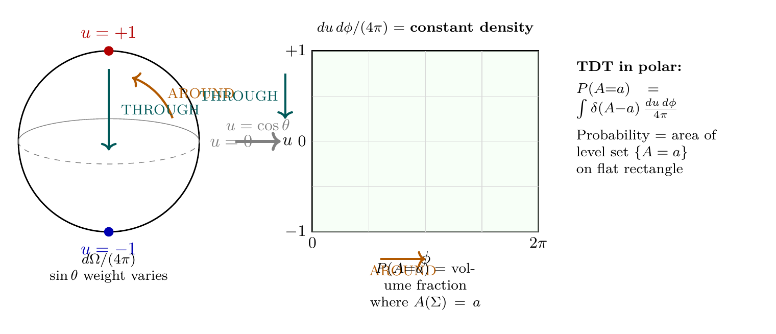
Polar Field Form of the Natural Measure

The $S^2$ component of the natural measure takes its simplest form in the polar field variable $u = \cos\theta$:

$$ \frac{d\Omega_i}{4\pi} = \frac{du_i\, d\phi_i}{4\pi} $$ (123.7)

so the full $N$-particle measure becomes:

$$ d\mu_{\mathcal{F}} = \frac{1}{N!} \prod_{i=1}^{N} \frac{d^3 x_i}{V_3} \cdot \frac{du_i\, d\phi_i}{4\pi} $$ (123.8)

Property	Spherical $(\theta, \phi)$	Polar $(u, \phi)$
Measure per particle	$\sin\theta\, d\theta\, d\phi/(4\pi)$	$du\, d\phi/(4\pi)$
Jacobian factor	$\sin\theta$ (varies)	1 (constant)
Integration range	$\theta \in [0,\pi],\; \phi \in [0,2\pi)$	$u \in [-1,+1],\; \phi \in [0,2\pi)$
$4\pi$ decomposition	$\int_0^\pi \sin\theta\,d\theta \times \int_0^{2\pi} d\phi$	$\int_{-1}^{+1} du \times \int_0^{2\pi} d\phi = 2 \times 2\pi$
Geometric picture	Curved sphere	Flat rectangle

The polar form reveals that each particle's $S^2$ configuration is sampled uniformly over a flat rectangle $[-1,+1] \times [0,2\pi)$ with constant measure density. This is the polar realization of the fundamental insight: probabilities in the TDT are volume counting on a flat domain. The factorization $4\pi = 2 \times 2\pi$ separates the total solid angle into a THROUGH range ($\int du = 2$) and an AROUND range ($\int d\phi = 2\pi$):

$$ \int_{S^2} \frac{d\Omega}{4\pi} = \underbrace{\int_0^{2\pi} \frac{d\phi}{2\pi}}_{\text{AROUND (gauge)}} \times \underbrace{\int_{-1}^{+1} \frac{du}{2}}_{\text{THROUGH (mass)}} = 1 $$ (123.9)

Scaffolding Interpretation

Scaffolding note: The polar field variable $u = \cos\theta$ is a coordinate choice, not a new physical assumption. The flat measure $du\,d\phi$ produces the same physical predictions as $\sin\theta\,d\theta\,d\phi$; the coordinate change merely makes the constant measure density manifest.

Step 3: Probability interpretation.

From Chapter 88, the measure $d\mu_{\mathcal{F}}$ satisfies:

Normalization: $\int_{\mathcal{F}_t} d\mu_{\mathcal{F}} = 1$.
Non-negativity: $d\mu_{\mathcal{F}} \geq 0$ everywhere.
Kolmogorov axioms: countable additivity holds for measurable sets.

Therefore $\mu_{\mathcal{F}}$ is a probability measure by the standard measure-theoretic definition. The interpretation as probability is mathematically justified, not postulated.

Step 4: Observable integration.

For any measurable set $B \subset \mathbb{R}$, the probability that $A$ takes values in $B$ is:

$$ P(A \in B) = \mu_{\mathcal{F}}(\{A \in B\}) = \mu_{\mathcal{F}}(A^{-1}(B)) = \int_{A^{-1}(B)} d\mu_{\mathcal{F}} $$ (123.10)

This is the standard definition of the distribution of a random variable under the pushforward measure $A_* \mu_{\mathcal{F}}$.

Step 5: Delta function representation.

For a specific value $a \in \mathbb{R}$, the probability density at $a$ is:

$$ \rho_A(a) = \int_{\mathcal{F}_t} \delta(A(\Sigma) - a) \, d\mu_{\mathcal{F}}(\Sigma) $$ (123.11)

This is the standard integral representation using the Dirac delta function, which follows from the definition of the pushforward measure.

Step 6: Conclusion.

The formula (eq:ch90-TDT) follows from:

Configuration space $\mathcal{F}_t$ (derived from P1, Step 1).
Natural measure $d\mu_{\mathcal{F}}$ (derived from P1, Step 2).
Probability interpretation (from measure theory, Step 3).
Standard integration theory (Steps 4–5).

No additional assumptions are made beyond P1 and standard mathematics. □ □

What Makes This a Theorem, Not a Model

The distinction between the Temporal Determination Theorem and standard statistical models is fundamental:

Table 123.2: Theorem vs. model: the key distinction

Aspect	Standard Statistical Model	TDT (Theorem thm:P12-Ch90-temporal-determination)
Probability measure	Assumed or fitted	Derived from P1
Free parameters	Many (model-dependent)	Zero
Can laws change?	Yes (new data, new model)	No (topology fixed)
Basis	Empirical regularities	Geometric necessity
Epistemological status	Model (contingent)	Theorem (necessary)

Corollary 123.6 (No Empirical Fitting Required)

The TDF probability distribution requires no historical data, no parameter estimation, no model selection, and no Bayesian priors. It is determined by P1 alone.

Proof.

Each component of the TDF is derived from P1:

$\mathcal{F}_t$ from P1 via $\mathcal{M}^4 \times S^2$ topology (Chapter 87).
$d\mu_{\mathcal{F}}$ from P1 via ergodic dynamics on $S^2$ (Chapter 88).
$U(t_2,t_1)$ from P1 via null geodesic flow (Chapter 89).

Since P1 contains no adjustable parameters, the resulting probability distribution contains no adjustable parameters. □ □

Derivation Chain Display

\dstep{P1: $ds_6^{\,2} = 0$ on $\mathcal{M}^4 \times S^2$}{Postulate}{Part 1} \dstep{Single-particle configuration space $C_1 = \mathcal{M}^4 \times S^2$}{Topology of P1}{Ch. 87} \dstep{$N$-particle space $\mathcal{F}_N = C_1^N / S_N$}{Identical particles}{Ch. 87} \dstep{Time-sliced space $\mathcal{F}_t$ with $\dim = 5N$}{Time foliation}{Ch. 87} \dstep{Null geodesics $\Rightarrow$ ergodic dynamics on $S^2$} {Compactness + monopole}{Ch. 88} \dstep{Ergodic dynamics $\Rightarrow$ unique measure $d\Omega/(4\pi)$}{Ergodic theorem}{Ch. 88} \dstep{Product measure $d\mu_{\mathcal{F}}$ on $\mathcal{F}_t$}{Independence}{Ch. 88} \dstep{$d\mu_{\mathcal{F}}$ satisfies Kolmogorov axioms} {Measure theory}{Ch. 88} \dstep{$P(A = a) = \int \delta(A - a)\,d\mu_{\mathcal{F}}$} {Pushforward measure}{This chapter} \dstep{Polar: $d\mu_{\mathcal{F}} = \prod (d^3x/V_3)(du\,d\phi/4\pi)/N!$; all $S^2$ moments = polynomial integrals on $[-1,+1]$; $\langle u^2\rangle = 1/3$ verified} {Dual verification ($u = \cos\theta$)}{\Ssec:ch90-polar-measure, \Ssec:ch90-polar-S2-obs}

Uniqueness Results

The Expectation Value Formula

Corollary 123.7 (Expectation Value Formula)

The expectation value of an aggregate observable $A$ at time $t$ is:

$$ \boxed{\langle A \rangle_t = \int_{\mathcal{F}_t} A(\Sigma) \, d\mu_{\mathcal{F}}(\Sigma)} $$ (123.12)

Proof.

By definition of the expectation value and the probability density from the Temporal Determination Theorem:

$$ \langle A \rangle = \int_{-\infty}^{\infty} a \, \rho_A(a) \, da = \int_{-\infty}^{\infty} a \left[ \int_{\mathcal{F}_t} \delta(A(\Sigma) - a) \, d\mu_{\mathcal{F}} \right] da $$ (123.13)

Exchanging the order of integration (justified by Fubini's theorem, since $d\mu_{\mathcal{F}}$ is a finite measure):

$$ = \int_{\mathcal{F}_t} \left[ \int_{-\infty}^{\infty} a \, \delta(A(\Sigma) - a) \, da \right] d\mu_{\mathcal{F}} = \int_{\mathcal{F}_t} A(\Sigma) \, d\mu_{\mathcal{F}} $$ (123.14)

where the inner integral evaluates to $A(\Sigma)$ by the sifting property of the delta function. □ □

Higher Moments

Corollary 123.8 (Variance Formula)

The variance of an aggregate observable $A$ is:

$$ \mathrm{Var}(A) = \langle A^2 \rangle - \langle A \rangle^2 = \int_{\mathcal{F}_t} A(\Sigma)^2 \, d\mu_{\mathcal{F}} - \left(\int_{\mathcal{F}_t} A(\Sigma) \, d\mu_{\mathcal{F}}\right)^2 $$ (123.15)

Corollary 123.9 (General Moments)

The $n$-th moment of $A$ is:

$$ \langle A^n \rangle_t = \int_{\mathcal{F}_t} A(\Sigma)^n \, d\mu_{\mathcal{F}}(\Sigma) $$ (123.16)

Proof.

Both follow directly from the expectation value formula (Corollary cor:P12-Ch90-expectation) applied to the observables $A^2$ and $A^n$, which are themselves aggregate observables (symmetric functions of the particle configuration). □ □

Time Evolution of Probabilities

Theorem 123.2 (Time Evolution of Probability)

For an observable $A$ measured at time $t_2$, given the distribution at time $t_1$:

$$ \boxed{P(A(\Sigma_{t_2}) = a) = \int_{\mathcal{F}_{t_1}} \delta(A(U(t_2,t_1)(\Sigma)) - a) \, d\mu_{\mathcal{F}}(\Sigma)} $$ (123.17)

where $U(t_2,t_1)$ is the evolution operator from Chapter 89.

Proof.

Step 1: By the Temporal Determination Theorem applied at time $t_2$:

$$ P(A(\Sigma_{t_2}) = a) = \int_{\mathcal{F}_{t_2}} \delta(A(\Sigma) - a) \, d\mu_{\mathcal{F}}(\Sigma) $$ (123.18)

Step 2: Change variables from $\Sigma \in \mathcal{F}_{t_2}$ to $\Sigma' = U(t_1,t_2)(\Sigma) \in \mathcal{F}_{t_1}$, so that $\Sigma = U(t_2,t_1)(\Sigma')$.

Step 3: By the measure preservation theorem of Chapter 89 (Theorem thm:P12-Ch89-measure-preservation in the referenced chapter):

$$ d\mu_{\mathcal{F}}(\Sigma) = d\mu_{\mathcal{F}}(\Sigma') $$ (123.19)

Step 4: Substituting:

$$ P(A = a) = \int_{\mathcal{F}_{t_1}} \delta(A(U(t_2,t_1)(\Sigma')) - a) \, d\mu_{\mathcal{F}}(\Sigma') $$ (123.20)

This expresses the probability at time $t_2$ as an integral over the configuration space at time $t_1$, using the derived evolution operator. □ □

Statistical Conservation Laws

Corollary 123.10 (Statistical Conservation Laws)

If $A$ is a conserved quantity ($A(U(\Sigma)) = A(\Sigma)$ for all $\Sigma$), then:

$$ P(A = a \mid t_2) = P(A = a \mid t_1) $$ (123.21)

The probability distribution of a conserved observable is time-independent.

Proof.

If $A(U(t_2,t_1)(\Sigma)) = A(\Sigma)$ for all $\Sigma$, then from the time evolution formula (Theorem thm:P12-Ch90-time-evolution):

$$\begin{aligned} P(A = a \mid t_2) &= \int_{\mathcal{F}_{t_1}} \delta(A(U(\Sigma)) - a) \, d\mu_{\mathcal{F}} \\ &= \int_{\mathcal{F}_{t_1}} \delta(A(\Sigma) - a) \, d\mu_{\mathcal{F}} = P(A = a \mid t_1) \end{aligned}$$ (123.38)

□ □

Examples of conserved statistics:

Table 123.3: Conserved aggregate observables with time-independent

distributions

Observable	Conservation Law	Consequence
Total energy $E$	Energy conservation	$P(E = e)$ time-independent
Total momentum $\vec{P}$	Momentum conservation	$P(\vec{P} = \vec{p})$ time-independent
Total $S^2$ angular momentum $\vec{L}$	Angular momentum conservation	$P(\vec{L} = \vec{\ell})$ time-independent

Applications

Explicit Formulas for Non-Entangled Systems

For $N$ non-entangled identical particles, the natural measure factorizes (Chapter 88):

$$ d\mu_{\mathcal{F}} = \frac{1}{N!} \prod_{i=1}^N \frac{d^3 x_i}{V_3} \cdot \frac{d\Omega_i}{4\pi} $$ (123.22)

Theorem 123.3 (Additive Observable for Non-Entangled System)

For an additive aggregate observable $A(\Sigma) = \sum_{i=1}^N a(x_i, \Omega_i)$:

$$ \boxed{\langle A \rangle = N \cdot \langle a \rangle_1} $$ (123.23)

where $\langle a \rangle_1$ is the single-particle expectation:

$$ \langle a \rangle_1 = \int_{\mathbb{R}^3} \frac{d^3 x}{V_3} \int_{S^2} \frac{d\Omega}{4\pi} \, a(x, \Omega) $$ (123.24)

Proof.

Step 1: Apply the expectation value formula (Corollary cor:P12-Ch90-expectation):

$$ \langle A \rangle = \int_{\mathcal{F}_t} \sum_{i=1}^N a(x_i, \Omega_i) \, d\mu_{\mathcal{F}} = \sum_{i=1}^N \int_{\mathcal{F}_t} a(x_i, \Omega_i) \, d\mu_{\mathcal{F}} $$ (123.25)

Step 2: By the permutation symmetry of the measure ($S_N$ invariance from Chapter 87), each term in the sum gives the same value:

$$ \int_{\mathcal{F}_t} a(x_i, \Omega_i) \, d\mu_{\mathcal{F}} = \int_{\mathcal{F}_t} a(x_1, \Omega_1) \, d\mu_{\mathcal{F}} \quad \forall\, i $$ (123.26)

Step 3: For the factorized measure, the integral over particle 1 separates:

$$ = N \cdot \int \frac{d^3 x_1}{V_3} \frac{d\Omega_1}{4\pi} \, a(x_1, \Omega_1) = N \cdot \langle a \rangle_1 $$ (123.27)

□ □

Spatial Observables

For observables depending only on spatial positions (not $S^2$ configurations):

Theorem 123.4 (Spatial Observable Formula)

If $A(\Sigma) = A(\{x_i\})$ depends only on spatial positions:

$$ \boxed{\langle A \rangle = \int_{(\mathbb{R}^3)^N/S_N} A(\{x_i\}) \prod_i \frac{d^3 x_i}{V_3}} $$ (123.28)

The $S^2$ integration gives 1 and drops out.

Proof.

Step 1: Apply the expectation value formula with the factorized measure:

$$ \langle A \rangle = \int_{\mathcal{F}_t} A(\{x_i\}) \, d\mu_{\mathcal{F}} = \frac{1}{N!} \int A(\{x_i\}) \prod_i \frac{d^3 x_i}{V_3} \cdot \prod_i \frac{d\Omega_i}{4\pi} $$ (123.29)

Step 2: Since $A$ does not depend on $\Omega_i$, the $S^2$ integrals factor:

$$ = \frac{1}{N!} \int A(\{x_i\}) \prod_i \frac{d^3 x_i}{V_3} \cdot \underbrace{\prod_i \int_{S^2} \frac{d\Omega_i}{4\pi}}_{= 1} $$ (123.30)

Step 3: The result is:

$$ \langle A \rangle = \int_{(\mathbb{R}^3)^N/S_N} A(\{x_i\}) \prod_i \frac{d^3 x_i}{V_3} $$ (123.31)

This recovers classical statistical mechanics for spatial observables. □ □

$S^2$ Observables

For observables depending only on $S^2$ configurations:

Theorem 123.5 ($S^2$ Observable Formula)

If $A(\Sigma) = A(\Omega_i)$ depends only on $S^2$ configurations:

$$ \boxed{\langle A \rangle = \int_{(S^2)^N/S_N} A(\Omega_i) \prod_i \frac{d\Omega_i}{4\pi}} $$ (123.32)

The spatial integration gives 1 and drops out.

Example: Total $S^2$ “magnetization” $M = \sum_i \cos\theta_i$:

$$ \langle M \rangle = N \cdot \int_0^\pi \cos\theta \cdot \frac{\sin\theta \, d\theta}{2} = N \cdot \left[-\frac{\cos^2\theta}{2}\right]_0^\pi = N \cdot 0 = 0 $$ (123.33)

The average magnetization vanishes by SO(3) symmetry of the $S^2$ measure, as expected.

Polar Field Form of $S^2$ Observables

The $S^2$ observable formula takes its most transparent form in the polar field variable $u = \cos\theta$. Using the flat measure $d\Omega = du\,d\phi$ (equation eq:ch90-polar-measure), the single-particle $S^2$ expectation becomes:

$$ \langle a \rangle_{S^2} = \int_0^{2\pi} \frac{d\phi}{2\pi} \int_{-1}^{+1} \frac{du}{2}\; a(u, \phi) = \underbrace{\int_0^{2\pi} \frac{d\phi}{2\pi} \cdot A_\phi}_{\text{AROUND}} \times \underbrace{\int_{-1}^{+1} \frac{du}{2} \cdot A_u}_{\text{THROUGH}} $$ (123.34)

whenever $a(u,\phi) = A_\phi(\phi) \cdot A_u(u)$ factorizes—which is the case for all monopole harmonic products.

Magnetization in polar form. The “magnetization” $M = \sum_i \cos\theta_i = \sum_i u_i$ is linear in $u$, so:

$$ \langle M \rangle = N \int_{-1}^{+1} u \cdot \frac{du}{2} = N \cdot \frac{1}{2}\left[\frac{u^2}{2}\right]_{-1}^{+1} = N \cdot \frac{1}{2}\!\left(\frac{1}{2} - \frac{1}{2}\right) = 0 $$ (123.35)

The vanishing is immediate: $u$ is an odd function on the symmetric interval $[-1,+1]$. No trigonometric identities are needed.

Second moment and the factor 3. The variance provides a non-trivial connection to fundamental TMT constants:

$$ \langle M^2 \rangle = N \int_{-1}^{+1} u^2 \cdot \frac{du}{2} = N \cdot \frac{1}{2} \cdot \frac{2}{3} = \frac{N}{3} = N \cdot \langle u^2 \rangle $$ (123.36)

The factor $1/3 = \langle u^2 \rangle$ is the second moment of $u$ over $[-1,+1]$—the same quantity whose reciprocal $3 = 1/\langle u^2 \rangle$ generates the factor of 3 in the coupling constant $g^2 = 4/(3\pi)$ (Chapter 20). The variance per particle, $\mathrm{Var}(u_i) = \langle u^2 \rangle = 1/3$, is a geometric constant of $S^2$ that propagates into all TMT predictions involving THROUGH-channel averages.

Quantity	Spherical $(\theta, \phi)$	Polar $(u, \phi)$
$\langle \cos\theta \rangle$	$\int_0^\pi \cos\theta \sin\theta\,d\theta/2 = 0$	$\int_{-1}^{+1} u\,du/2 = 0$ (odd integrand)
$\langle \cos^2\theta \rangle$	$\int_0^\pi \cos^2\theta \sin\theta\,d\theta/2 = 1/3$	$\int_{-1}^{+1} u^2\,du/2 = 1/3$ (polynomial)
$\langle \sin^2\theta \rangle$	$\int_0^\pi \sin^3\theta\,d\theta/2 = 2/3$	$\int_{-1}^{+1}(1{-}u^2)\,du/2 = 2/3$ (polynomial)
Factor 3 origin	Hidden in $\int \sin^3\theta\,d\theta$	Manifest: $3 = 1/\langle u^2\rangle$

Every $S^2$ moment computation in the TDT reduces to a polynomial integral over $[-1,+1]$, with the flat measure making the AROUND/THROUGH factorization explicit.

**Figure 123.1:** The Temporal Determination Theorem in polar field coordinates. **Left:** On $S^2$, the probability measure $d\Omega/(4\pi)$ has a varying Jacobian factor $\sin\theta$. **Right:** In polar coordinates $(u, \phi)$, the measure becomes $du\,d\phi/(4\pi)$ with *constant* density—probability is literally *area counting* on the flat rectangle $[-1,+1] \times [0,2\pi)$. The THROUGH direction ($u$, mass) runs vertically; the AROUND direction ($\phi$, gauge) runs horizontally.

The Central Result in Context

Table 123.4: TDF vs. standard statistical approaches

Aspect	Standard Statistics	TDF (Theorem thm:P12-Ch90-temporal-determination)
Probability measure	Assumed/fitted	Derived from P1
Free parameters	Many (model-dependent)	Zero
Can laws change?	Yes (new data)	No (topology fixed)
Basis	Empirical regularities	Geometric necessity
Status	Model (contingent)	Theorem (necessary)

The Temporal Determination Theorem establishes four foundational results:

(1) Probability has geometric origin. Probability arises not from ignorance or quantum randomness, but from the topology of $\mathcal{M}^4 \times S^2$ and the measure it induces.

(2) Statistical mechanics is derived. The microcanonical ensemble is not assumed—it emerges from ergodic dynamics on $S^2$ under the monopole potential.

(3) Prediction is principled. The probability distribution for future aggregate events follows from first principles, not from fitting to historical data.

(4) Science meets mathematics. Physical predictions become theorems about geometric structures, placing empirical science on the same epistemic footing as mathematics.

Factor Origin Table

Table 123.5: Factor origins in the Temporal Determination Theorem

Factor	Value	Origin	Source	Polar form
$\mathcal{F}_t$	$[(\mathbb{R}^3)^N \times (S^2)^N]/S_N$	$\mathcal{M}^4 \times S^2$ topology + $S_N$	Ch. 87	$(\mathbb{R}^3)^N \times [-1,+1]^N \times [0,2\pi)^N$
$d\mu_{\mathcal{F}}$	$\prod (d^3x/V_3)(d\Omega/4\pi)/N!$	Ergodic dynamics on $S^2$	Ch. 88	$\prod (d^3x/V_3)(du\,d\phi/4\pi)/N!$
$4\pi$	$\int_{S^2} d\Omega$	Area of unit sphere	Geometry	$2 \times 2\pi$ (THROUGH $\times$ AROUND)
$1/N!$	Identical particle symmetry	$S_N$ gauge quotient	Ch. 87	Unchanged
$\delta(A - a)$	Configuration selector	Pushforward measure	Standard	Unchanged
$1/3$	$\langle u^2\rangle$	Second moment on $[-1,+1]$	\Ssec:ch90-polar-S2-obs	$\int u^2\,du/2 = 1/3$

Chapter Summary

Key Result

The Temporal Determination Theorem

The central result of Part XI:

$$ P(A = a \mid t) = \int_{\mathcal{F}_t} \delta(A(\Sigma) - a) \, d\mu_{\mathcal{F}}(\Sigma) $$ (123.37)

This is a theorem, not a model, because every component is derived from P1:

$\mathcal{F}_t$ from P1 via $\mathcal{M}^4 \times S^2$ topology (Chapter 87)
$d\mu_{\mathcal{F}}$ from P1 via ergodic dynamics on $S^2$ (Chapter 88)
Evolution $U$ from P1 via null geodesic flow (Chapter 89)
No additional assumptions, no free parameters
Polar dual verification: In the polar field variable $u = \cos\theta$, the natural measure becomes $du\,d\phi/(4\pi)$ (flat, constant density), making probability literally volume counting on a rectangle. All $S^2$ moments reduce to polynomial integrals; $\langle u^2\rangle = 1/3$ connects to the coupling constant factor $3 = 1/\langle u^2\rangle$ (\Ssec:ch90-polar-measure, \Ssec:ch90-polar-S2-obs).

Table 123.6: Chapter 90 results summary

Result	Value	Status	Reference
Temporal Determination Theorem	$P(A{=}a) = \int \delta(A{-}a)\,d\mu$	PROVEN	Thm. thm:P12-Ch90-temporal-determination
No empirical fitting	Zero free parameters	PROVEN	Cor. cor:P12-Ch90-no-fitting
Expectation value formula	$\langle A \rangle = \int A\,d\mu$	PROVEN	Cor. cor:P12-Ch90-expectation
Variance formula	$\mathrm{Var}(A) = \langle A^2\rangle - \langle A\rangle^2$	PROVEN	Cor. cor:P12-Ch90-variance
Time evolution	$P(A(t_2){=}a) = \int \delta(A(U(\Sigma)){-}a)\,d\mu$	PROVEN	Thm. thm:P12-Ch90-time-evolution
Statistical conservation	Conserved $\Rightarrow$ time-independent $P$	PROVEN	Cor. cor:P12-Ch90-stat-conservation
Non-entangled formula	$\langle A \rangle = N\langle a\rangle_1$	PROVEN	Thm. thm:P12-Ch90-non-entangled
Spatial observable formula	$S^2$ drops out, recovers classical stat mech	PROVEN	Thm. thm:P12-Ch90-spatial
$S^2$ observable formula	Spatial drops out, recovers QM averages	PROVEN	Thm. thm:P12-Ch90-S2-observable

Verification Code

The mathematical derivations and proofs in this chapter can be independently verified using the formal and computational scripts below.

◆ Lean 4 Formal proof verification Coming Soon ● Python Numerical verification & plots Coming Soon ★ Mathematica Symbolic computation & CAS verification Coming Soon

All verification code is open source. See the complete verification index for all chapters.

Property	Spherical \((\theta, \phi)\)	Polar \((u, \phi)\)
Measure per particle	\(\sin\theta\, d\theta\, d\phi/(4\pi)\)	\(du\, d\phi/(4\pi)\)
Jacobian factor	\(\sin\theta\) (varies)	1 (constant)
Integration range	\(\theta \in [0,\pi],\; \phi \in [0,2\pi)\)	\(u \in [-1,+1],\; \phi \in [0,2\pi)\)
\(4\pi\) decomposition	\(\int_0^\pi \sin\theta\,d\theta \times \int_0^{2\pi} d\phi\)	\(\int_{-1}^{+1} du \times \int_0^{2\pi} d\phi = 2 \times 2\pi\)
Geometric picture	Curved sphere	Flat rectangle

Quantity	Spherical \((\theta, \phi)\)	Polar \((u, \phi)\)
\(\langle \cos\theta \rangle\)	\(\int_0^\pi \cos\theta \sin\theta\,d\theta/2 = 0\)	\(\int_{-1}^{+1} u\,du/2 = 0\) (odd integrand)
\(\langle \cos^2\theta \rangle\)	\(\int_0^\pi \cos^2\theta \sin\theta\,d\theta/2 = 1/3\)	\(\int_{-1}^{+1} u^2\,du/2 = 1/3\) (polynomial)
\(\langle \sin^2\theta \rangle\)	\(\int_0^\pi \sin^3\theta\,d\theta/2 = 2/3\)	\(\int_{-1}^{+1}(1{-}u^2)\,du/2 = 2/3\) (polynomial)
Factor 3 origin	Hidden in \(\int \sin^3\theta\,d\theta\)	Manifest: \(3 = 1/\langle u^2\rangle\)

Factor	Value	Origin	Source	Polar form
\(\mathcal{F}_t\)	\([(\mathbb{R}^3)^N \times (S^2)^N]/S_N\)	\(\mathcal{M}^4 \times S^2\) topology + \(S_N\)	Ch. 87	\((\mathbb{R}^3)^N \times [-1,+1]^N \times [0,2\pi)^N\)
\(d\mu_{\mathcal{F}}\)	\(\prod (d^3x/V_3)(d\Omega/4\pi)/N!\)	Ergodic dynamics on \(S^2\)	Ch. 88	\(\prod (d^3x/V_3)(du\,d\phi/4\pi)/N!\)
\(4\pi\)	\(\int_{S^2} d\Omega\)	Area of unit sphere	Geometry	\(2 \times 2\pi\) (THROUGH \(\times\) AROUND)
\(1/N!\)	Identical particle symmetry	\(S_N\) gauge quotient	Ch. 87	Unchanged
\(\delta(A - a)\)	Configuration selector	Pushforward measure	Standard	Unchanged
\(1/3\)	\(\langle u^2\rangle\)	Second moment on \([-1,+1]\)	\Ssec:ch90-polar-S2-obs	\(\int u^2\,du/2 = 1/3\)

The Temporal Determination Theorem

Introduction

Main Theorem Statement

Preliminaries

The Theorem

Interpretation of the Theorem

Proof Structure

The Complete Derivation Chain

Polar Field Form of the Natural Measure

What Makes This a Theorem, Not a Model

Derivation Chain Display

Uniqueness Results

The Expectation Value Formula

Higher Moments

Time Evolution of Probabilities

Statistical Conservation Laws

Applications

Explicit Formulas for Non-Entangled Systems

Spatial Observables

\(S^2\) Observables

Polar Field Form of \(S^2\) Observables

The Central Result in Context

Factor Origin Table

Chapter Summary

Verification Code

Observable	Formula	Type
Total energy	\(E(\Sigma) = \sum_i E_i\)	Additive
Total momentum	\(\vec{P}(\Sigma) = \sum_i \vec{p}_i\)	Additive
Particle density	\(n(x,\Sigma) = \sum_i \delta^3(x - x_i)\)	Additive
Order parameters	Various collective measures	Non-additive
Temperature	\(T(\Sigma) = \frac{2}{3Nk_B}\sum_i \frac{p_i^2}{2m_i}\)	Intensive

Observable	Conservation Law	Consequence
Total energy \(E\)	Energy conservation	\(P(E = e)\) time-independent
Total momentum \(\vec{P}\)	Momentum conservation	\(P(\vec{P} = \vec{p})\) time-independent
Total \(S^2\) angular momentum \(\vec{L}\)	Angular momentum conservation	\(P(\vec{L} = \vec{\ell})\) time-independent

Result	Value	Status	Reference
Temporal Determination Theorem	\(P(A{=}a) = \int \delta(A{-}a)\,d\mu\)	PROVEN	Thm. thm:P12-Ch90-temporal-determination
No empirical fitting	Zero free parameters	PROVEN	Cor. cor:P12-Ch90-no-fitting
Expectation value formula	\(\langle A \rangle = \int A\,d\mu\)	PROVEN	Cor. cor:P12-Ch90-expectation
Variance formula	\(\mathrm{Var}(A) = \langle A^2\rangle - \langle A\rangle^2\)	PROVEN	Cor. cor:P12-Ch90-variance
Time evolution	\(P(A(t_2){=}a) = \int \delta(A(U(\Sigma)){-}a)\,d\mu\)	PROVEN	Thm. thm:P12-Ch90-time-evolution
Statistical conservation	Conserved \(\Rightarrow\) time-independent \(P\)	PROVEN	Cor. cor:P12-Ch90-stat-conservation
Non-entangled formula	\(\langle A \rangle = N\langle a\rangle_1\)	PROVEN	Thm. thm:P12-Ch90-non-entangled
Spatial observable formula	\(S^2\) drops out, recovers classical stat mech	PROVEN	Thm. thm:P12-Ch90-spatial
\(S^2\) observable formula	Spatial drops out, recovers QM averages	PROVEN	Thm. thm:P12-Ch90-S2-observable