Chapter 15

Gauge Symmetry from Geometry

Introduction

With the interpretive framework established (Chapter 14), we now turn to the most remarkable consequence of $S^2$ geometry: gauge symmetry is not assumed — it is derived.

In the Standard Model, the gauge group $\text{SU}(3) \times \text{SU}(2) \times \text{U}(1)$ is a postulate. No explanation is given for why nature chose this particular group, why it has three factors, or why the dimensions are 8, 3, and 1 respectively. The gauge group is one of the Standard Model's $\sim$19 free parameters.

In TMT, the gauge group follows from geometry. The $S^2$ projection structure has three mathematical properties — isometry, topology, and embedding — that generate the three gauge group factors. This chapter begins with the first and most direct: isometry generates $\text{SU}(2)$.

Key Result

The Kaluza-Klein mechanism: When a space has continuous symmetries (isometries), the null constraint $ds_6^{\,2} = 0$ forces those symmetries to appear as gauge symmetries in 4D. On $S^2$, the isometry group is SO(3) $\cong$ SU(2)$/\mathbb{Z}_{2}$, so the 4D theory automatically contains SU(2) gauge bosons.

Derivation chain for this chapter:

P1 ($ds_6^{\,2} = 0$) $\to$ $S^2$ topology required (Ch. 8) $\to$ Iso($S^2$) $=$ SO(3) (this chapter) $\to$ Killing vectors $\xi_{a}$ (this chapter) $\to$ Gauge field $A_{\mu}^{a}$ (this chapter) $\to$ SU(2) gauge symmetry (this chapter)

Scaffolding Interpretation

Interpretation note (Chapter 14): The Kaluza-Klein mechanism works identically under both Interpretations A and B. Under Interpretation A, isometries are physical rotations of extra-dimensional space. Under Interpretation B, isometries are symmetries of the projection structure. The mathematical derivation — and therefore the gauge group — is the same in both cases.

The Kaluza-Klein Mechanism

The Kaluza-Klein mechanism is the mathematical procedure by which continuous symmetries of the internal space become gauge symmetries in the effective 4D theory. We present it here in the TMT context: the $ds_6^{\,2} = 0$ constraint on $\mathcal{M}^4 \times S^2$ naturally produces gauge fields.

The General Principle

Theorem 15.1 (Kaluza-Klein Gauge Mechanism)

Let $(M^{D}, g_{AB})$ be a $D$-dimensional spacetime with a product structure $M^{D} = M^{d} \times K^{n}$, where $K^{n}$ is a compact manifold with isometry group $G = \text{Iso}(K^{n})$. Then:

The off-diagonal components $g_{\mu m}$ of the higher-dimensional metric decompose as:

$$ g_{\mu m}(x, y) = A_{\mu}^{a}(x)\,\xi_{a\,m}(y) $$ (15.1)

Under an isometry $y \to \phi(y)$ of $K^{n}$, the fields $A_{\mu}^{a}$ transform as gauge fields:

$$ A_{\mu}^{a} \to A_{\mu}^{a} + \partial_{\mu}\Lambda^{a} + f^{a}_{bc}\,A_{\mu}^{b}\,\Lambda^{c} $$ (15.2)

The gauge field strength is:

$$ F_{\mu\nu}^{a} = \partial_{\mu}A_{\nu}^{a} - \partial_{\nu}A_{\mu}^{a} + f^{a}_{bc}\,A_{\mu}^{b}\,A_{\nu}^{c}. $$ (15.3)

Proof.

This is a standard result in Kaluza-Klein theory, established by Kaluza (1921), Klein (1926), and developed systematically by DeWitt (1964), Kerner (1968), and Cho (1975).

Step 1 (Metric ansatz): The most general metric on $M^{d} \times K^{n}$ compatible with $d$-dimensional Poincar\’{e} invariance is:

$$ ds_{D}^{2} = g_{\mu\nu}(x)\,dx^{\mu}dx^{\nu} + g_{mn}(y)\bigl(dy^{m} + A_{\mu}^{a}\xi_{a}^{m}\,dx^{\mu}\bigr)\bigl(dy^{n} + A_{\nu}^{b}\xi_{b}^{n}\,dx^{\nu}\bigr). $$ (15.4)

Step 2 (Gauge transformation): An infinitesimal isometry $y^{m} \to y^{m} + \epsilon^{a}\xi_{a}^{m}(y)$ leaves $g_{mn}$ invariant (by definition of Killing vectors) but shifts $A_{\mu}^{a}$:

$$ \delta A_{\mu}^{a} = \partial_{\mu}\epsilon^{a} + f^{a}_{bc}\,A_{\mu}^{b}\,\epsilon^{c}. $$ (15.5)

This is exactly a non-abelian gauge transformation with parameter $\epsilon^{a}(x)$.

Step 3 (Field strength): The Riemann tensor $R_{ABCD}$ of $ds_{D}^{2}$ contains the field strength $F_{\mu\nu}^{a}$ in its $(\mu\nu mn)$ components, confirming the gauge structure.

(See: Part 3 §7.4.1; Kaluza (1921); Klein (1926)) □

Application to TMT

For TMT with $D = 6$, $d = 4$, $K^{2} = S^2$:

Table 15.1: Kaluza-Klein mechanism applied to TMT

General KK	TMT Specification	Result
$K^{n}$	$S^2$	Compact projection structure
$G = \text{Iso}(K^{n})$	Iso($S^2$) $=$ SO(3)	Three-dimensional symmetry group
$\dim(G)$	3	Three gauge fields
$\xi_{a}$	Three Killing vectors on $S^2$	Generators of SO(3) rotations
$A_{\mu}^{a}$	Three gauge bosons	$W^{1}_{\mu}$, $W^{2}_{\mu}$, $W^{3}_{\mu}$
$f^{a}_{bc}$	$\epsilon_{abc}$	$\mathfrak{su}(2)$ structure constants

Key Result

Key point: The number of gauge bosons (3) is not chosen — it equals $\dim(\text{Iso}(S^2)) = \dim(\text{SO}(3)) = 3$. This is a geometric fact about the 2-sphere, not an input parameter.

Isometries Become Gauge Symmetries

Definition of Isometry

Definition 15.10 (Isometry)

An isometry of a Riemannian manifold $(M, g)$ is a diffeomorphism $\phi: M \to M$ that preserves the metric:

$$ \phi^{*}g = g. $$ (15.6)

The set of all isometries forms a Lie group called the isometry group $\text{Iso}(M)$.

Isometry Group of $S^2$

Theorem 15.2 (Isometry Group of $S^2$)

The isometry group of the round 2-sphere $(S^2, R^{2}(d\theta^{2} + \sin^{2}\theta\,d\phi^{2}))$ is:

$$ \text{Iso}(S^2) = \text{O}(3). $$ (15.7)

The connected component containing the identity is:

$$ \text{Iso}_{0}(S^2) = \text{SO}(3). $$ (15.8)

The dimension of the isometry group is:

$$ \dim\bigl(\text{Iso}(S^2)\bigr) = \dim\bigl(\text{SO}(3)\bigr) = 3. $$ (15.9)

This is the maximum possible dimension for the isometry group of any 2-dimensional manifold. A Riemannian $n$-manifold has at most $n(n+1)/2$ independent Killing vectors; for $n = 2$ this is $2(3)/2 = 3$. The 2-sphere saturates this bound.

Proof.

Step 1: The round 2-sphere is defined as $S^2 = \{x \in \mathbb{R}^{3} : |x| = R\}$ with the metric induced from $\mathbb{R}^{3}$.

Step 2: Every orthogonal transformation $O \in \text{O}(3)$ maps $S^2$ to itself (preserves $|x| = R$) and preserves the induced metric (the Euclidean inner product is O(3)-invariant).

Step 3: Conversely, every isometry of $S^2$ extends uniquely to an orthogonal transformation of $\mathbb{R}^{3}$. This follows from the rigidity of the sphere: a distance-preserving map of $S^2$ must preserve all angles and therefore must be a rotation or a rotation composed with a reflection.

Step 4: Therefore $\text{Iso}(S^2) = \text{O}(3)$, and the identity component is $\text{SO}(3)$.

Step 5: $\dim(\text{SO}(3)) = 3$ (three independent rotation axes), which equals the maximum $n(n+1)/2 = 3$ for $n = 2$.

(See: Part 3 §7.1.2) □

Why This Matters for Gauge Physics

The fact that Iso($S^2$) $=$ SO(3) has three immediate consequences for physics:

Number of gauge bosons: There are exactly 3 generators, hence exactly 3 gauge bosons. In the Standard Model, these become $W^{1}$, $W^{2}$, $W^{3}$ (the SU(2) triplet).

Non-abelian structure: SO(3) is non-abelian ($[R_{x}, R_{y}] \neq 0$), so the gauge theory is non-abelian. This is essential for the weak force — an abelian gauge group (like U(1)) could not produce the charged current interactions observed in beta decay.

Maximality: $S^2$ has the maximum number of Killing vectors for a 2-manifold. This means TMT extracts the most gauge symmetry possible from two compact dimensions. No information is wasted.

Counterfactual: What if $K^{2}$ were not $S^2$?

Table 15.2: Gauge groups from alternative 2-manifolds

Manifold	Iso Group	dim(Iso)	Problem
$S^2$	SO(3)	3	None — correct
$T^{2}$ (torus)	U(1)$\times$U(1)	2	Abelian only; no weak force
$\Sigma_{g}$ ($g \geq 2$)	Finite	0	No continuous gauge symmetry
$\mathbb{RP}^{2}$	SO(3)	3	Same locally, wrong global topology

Only $S^2$ gives a non-abelian gauge group of the correct dimension from a compact 2-manifold.

(See: Part 3 §7.0.3)

Killing Vectors on $S^2$

The three Killing vectors on $S^2$ are the infinitesimal generators of SO(3) rotations. They are the mathematical objects that, through the Kaluza-Klein mechanism, become the gauge fields.

Definition of Killing Vector Fields

Definition 15.11 (Killing Vector Field)

A Killing vector field $\xi$ on a Riemannian manifold $(M, g)$ is an infinitesimal generator of isometries, satisfying the Killing equation:

$$ \nabla_{\mu}\xi_{\nu} + \nabla_{\nu}\xi_{\mu} = 0 $$ (15.10)

or equivalently, the Lie derivative of the metric vanishes:

$$ \mathcal{L}_{\xi}\,g = 0. $$ (15.11)

Geometrically, a Killing vector field generates a one-parameter family of isometries. The metric is invariant along the flow of $\xi$: distances and angles are unchanged as you move along $\xi$.

Explicit Killing Vectors on $S^2$

Theorem 15.3 (Killing Vectors on $S^2$)

The round 2-sphere $S^2$ with metric $ds^{2} = R^{2}(d\theta^{2} + \sin^{2}\theta\,d\phi^{2})$ has exactly three independent Killing vector fields, corresponding to rotations about the three Cartesian axes:

$$\begin{aligned} \xi_{1} &= -\sin\phi\,\partial_{\theta} - \cot\theta\,\cos\phi\,\partial_{\phi} \\ \xi_{2} &= \cos\phi\,\partial_{\theta} - \cot\theta\,\sin\phi\,\partial_{\phi} \\ \xi_{3} &= \partial_{\phi} \end{aligned}$$ (15.29)

These satisfy the $\mathfrak{so}(3)$ Lie algebra:

$$ \boxed{[\xi_{a}, \xi_{b}] = \epsilon_{abc}\,\xi_{c}} $$ (15.12)

where $\epsilon_{abc}$ is the Levi-Civita symbol.

Proof.

Step 1 (Killing equation): In coordinates $(\theta, \phi)$, the metric components are $g_{\theta\theta} = R^{2}$, $g_{\phi\phi} = R^{2}\sin^{2}\theta$, $g_{\theta\phi} = 0$. The Killing equation $\nabla_{\mu}\xi_{\nu} + \nabla_{\nu}\xi_{\mu} = 0$ gives three independent conditions:

$$\begin{aligned} (\theta\theta): \quad & \partial_{\theta}\xi^{\theta} = 0, \\ (\phi\phi): \quad & \partial_{\phi}\xi^{\phi} + \cos\theta\,\xi^{\theta}/\sin\theta = 0, \\ (\theta\phi): \quad & \sin^{2}\theta\,\partial_{\theta}\xi^{\phi} + \partial_{\phi}\xi^{\theta} = 0. \end{aligned}$$ (15.30)

Step 2 (Solution): From $(\theta\theta)$: $\xi^{\theta}$ is independent of $\theta$, so $\xi^{\theta} = f(\phi)$. From $(\phi\phi)$: $\partial_{\phi}\xi^{\phi} = -f(\phi)\cos\theta/\sin\theta$. From $(\theta\phi)$: the coupled system has general solution:

$$\begin{aligned} \xi^{\theta} &= A\cos\phi + B\sin\phi, \\ \xi^{\phi} &= C - (A\sin\phi - B\cos\phi)\cot\theta \end{aligned}$$ (15.31)

with three free constants $A$, $B$, $C$.

Step 3 (Basis choice): Setting $(A, B, C) = (0, -1, 0)$, $(1, 0, 0)$, $(0, 0, 1)$ gives $\xi_{1}$, $\xi_{2}$, $\xi_{3}$ respectively.

Step 4 (Lie bracket): Direct computation of $[\xi_{1}, \xi_{2}]$:

$$\begin{aligned} [\xi_{1}, \xi_{2}] &= \xi_{1}(\xi_{2}^{\theta})\partial_{\theta} + \xi_{1}(\xi_{2}^{\phi})\partial_{\phi} - \xi_{2}(\xi_{1}^{\theta})\partial_{\theta} - \xi_{2}(\xi_{1}^{\phi})\partial_{\phi} \\ &= \bigl(-\sin\phi\,\partial_{\theta}(\cos\phi) - \cot\theta\,\cos\phi\,\partial_{\phi}(\cos\phi)\bigr)\partial_{\theta} + \cdots \\ &= \partial_{\phi} = \xi_{3}. \end{aligned}$$ (15.32)

Similarly, $[\xi_{2}, \xi_{3}] = \xi_{1}$ and $[\xi_{3}, \xi_{1}] = \xi_{2}$, confirming $[\xi_{a}, \xi_{b}] = \epsilon_{abc}\,\xi_{c}$.

(See: Part 3 §7.2.2; Part 2 App 2A.1) □

Killing Vectors in Polar Field Coordinates

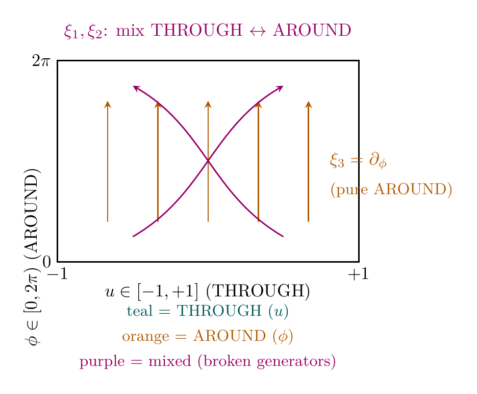
In the polar field variable $u = \cos\theta$ (Chapter 9), with $\partial_\theta = -(1-u^2)^{1/2}\,\partial_u$ and $\cot\theta = u/(1-u^2)^{1/2}$, the three Killing vectors become:

$$\begin{aligned} \xi_1 &= (1-u^2)^{1/2}\sin\phi\;\partial_u - \frac{u\cos\phi}{(1-u^2)^{1/2}}\;\partial_\phi \\ \xi_2 &= -(1-u^2)^{1/2}\cos\phi\;\partial_u - \frac{u\sin\phi}{(1-u^2)^{1/2}}\;\partial_\phi \\ \xi_3 &= \partial_\phi \end{aligned}$$ (15.33)

The polar form reveals the THROUGH/AROUND decomposition of gauge symmetry:

Table 15.3: Killing vectors: THROUGH/AROUND decomposition in polar coordinates

Killing Vector	THROUGH ($\partial_u$)	AROUND ($\partial_\phi$)	Mixing	Physics
$\xi_3$	0	$\partial_\phi$	Pure AROUND	Unbroken $U(1)_{\mathrm{em}}$
$\xi_1$	$(1-u^2)^{1/2}\sin\phi$	$-u\cos\phi/(1-u^2)^{1/2}$	Mixed	Broken $W^\pm$
$\xi_2$	$-(1-u^2)^{1/2}\cos\phi$	$-u\sin\phi/(1-u^2)^{1/2}$	Mixed	Broken $W^\pm$

Scaffolding Interpretation

Polar insight: The structure of electroweak symmetry breaking is visible in the coordinate decomposition. The unbroken generator $\xi_3 = \partial_\phi$ is pure AROUND — it moves only in the gauge direction, never touching the mass/gravity direction. The broken generators $\xi_1, \xi_2$ mix THROUGH and AROUND, coupling the $u$-direction (mass) to the $\phi$-direction (charge). Electroweak symmetry breaking, from the polar perspective, is the breaking of THROUGH-AROUND mixing while preserving the pure AROUND rotation.

Physical Interpretation of Each Killing Vector

Each Killing vector generates rotations about one Cartesian axis:

Table 15.4: Physical interpretation of $S^2$ Killing vectors

Killing Vector	Rotation Axis	Gauge Boson	Physical Role
$\xi_{1}$	$x$-axis	$W^{1}_{\mu}$	Charged current (with $\xi_{2}$)
$\xi_{2}$	$y$-axis	$W^{2}_{\mu}$	Charged current (with $\xi_{1}$)
$\xi_{3}$	$z$-axis	$W^{3}_{\mu}$	Neutral current (mixes with U(1))

After electroweak symmetry breaking, the physical gauge bosons are:

$$\begin{aligned} W^{\pm}_{\mu} &= \frac{1}{\sqrt{2}}\bigl(W^{1}_{\mu} \mp i\,W^{2}_{\mu}\bigr), \\ Z_{\mu} &= \cos\theta_{W}\,W^{3}_{\mu} - \sin\theta_{W}\,B_{\mu}, \\ A_{\mu} &= \sin\theta_{W}\,W^{3}_{\mu} + \cos\theta_{W}\,B_{\mu}, \end{aligned}$$ (15.34)

where $B_{\mu}$ is the U(1)$_{Y}$ gauge boson (derived in Chapter 17 from monopole topology) and $\theta_{W}$ is the Weinberg angle.

The Lie Algebra $\mathfrak{so}(3) \cong \mathfrak{su}(2)$

The commutation relations $[\xi_{a}, \xi_{b}] = \epsilon_{abc}\,\xi_{c}$ define the Lie algebra $\mathfrak{so}(3)$. This algebra is isomorphic to $\mathfrak{su}(2)$:

Theorem 15.4 (Lie Algebra Isomorphism)

The Lie algebras $\mathfrak{so}(3)$ and $\mathfrak{su}(2)$ are isomorphic:

$$ \mathfrak{so}(3) \cong \mathfrak{su}(2). $$ (15.13)

The isomorphism is given by:

$$ \xi_{a} \longleftrightarrow T_{a} = \frac{i\sigma_{a}}{2} $$ (15.14)

where $\sigma_{a}$ are the Pauli matrices:

$$\begin{aligned} \sigma_{1} = \begin{pmatrix} 0 & 1 \\ 1 & 0 \end{pmatrix}, \quad \sigma_{2} = \begin{pmatrix} 0 & -i \\ i & 0 \end{pmatrix}, \quad \sigma_{3} = \begin{pmatrix} 1 & 0 \\ 0 & -1 \end{pmatrix}. \end{aligned}$$ (15.15)

The generators $T_{a} = i\sigma_{a}/2$ satisfy:

$$ [T_{a}, T_{b}] = i\,\epsilon_{abc}\,T_{c}. $$ (15.16)

Proof.

Step 1: Both algebras have dimension 3.

Step 2: Both have structure constants $f_{abc} = \epsilon_{abc}$ (up to normalization conventions).

Step 3: The map $\xi_{a} \mapsto T_{a}$ preserves the bracket: $[\xi_{a}, \xi_{b}] = \epsilon_{abc}\,\xi_{c}$ maps to $[T_{a}, T_{b}] = i\,\epsilon_{abc}\,T_{c}$, where the factor of $i$ reflects the convention choice between real and complex generators.

Step 4: The map is bijective (both algebras are 3-dimensional, and the map sends a basis to a basis).

(See: Part 3 §7.3) □

The Double Cover Relation

Before considering fermions, we establish the fundamental relationship between SO(3) and SU(2):

Theorem 15.5 (Double Cover Relation: $\text{SU}(2) \to \text{SO}(3)$)

The group $\text{SU}(2)$ is the universal (double) cover of $\text{SO}(3)$:

$$ \text{SU}(2) \xrightarrow{\phi} \text{SO}(3) \xrightarrow{\text{quotient}} 1 $$ (15.17)

with kernel $\ker(\phi) = \mathbb{Z}_{2} = \pm I$ (the center of $\text{SU}(2)$).

Explicitly:

$$ \text{SO}(3) \cong \text{SU}(2)/\mathbb{Z}_{2}. $$ (15.18)

This means that every element of $\text{SO}(3)$ corresponds to exactly two elements of $\text{SU}(2)$, differing by a sign: $g$ and $-g$.

Proof.

Step 1 (Algebra isomorphism): Both $\text{SU}(2)$ and $\text{SO}(3)$ have Lie algebra $\mathfrak{so}(3) \cong \mathfrak{su}(2)$ with structure constants $\epsilon_{abc}$ (Theorem thm:P3-Ch15-lie-iso).

Step 2 (Explicit map): The map $\phi: \text{SU}(2) \to \text{SO}(3)$ is defined by the adjoint action: each element $g \in \text{SU}(2)$ acts on the Lie algebra by $v \mapsto gvg^{\dagger}$. This induces an $\text{SO}(3)$ action on the 3-dimensional vector space of traceless Hermitian matrices.

Step 3 (Kernel): The kernel consists of elements that act trivially: $gvg^\dagger} = v$ for all $v$. These are exactly the elements commuting with all of $\mathfrak{su}(2)$, which are the center $\{\pm I$.

Step 4 (Surjectivity): The map is surjective because every rotation in $\text{SO}(3)$ can be realized by conjugation of a Hermitian matrix by some $g \in \text{SU}(2)$.

Step 5 (Covering): Since $|\ker(\phi)| = 2$ and both groups have the same dimension (3), $\phi$ is a 2-to-1 covering map. $\text{SU}(2)$ is simply-connected (all its homotopy groups except $\pi_{1}$ vanish), making it the universal cover.

(See: Part 3 §7.3.1) □

The distinction between SO(3) and SU(2) becomes physically relevant when fermions are included:

Theorem 15.6 (SU(2) Required for Fermions)

The gauge group is $\text{SU}(2)$, not $\text{SO}(3)$, because:

Fermions (quarks and leptons) are observed in spin-$1/2$ representations.
Spin-$1/2$ (fundamental) representations exist for SU(2) but not for SO(3).
SO(3) has only integer-spin representations ($j = 0, 1, 2, \ldots$).
SU(2) additionally has half-integer-spin representations ($j = 1/2, 3/2, \ldots$).

Therefore, to accommodate fermions, the gauge group must be the universal cover $\text{SU}(2) = \widetilde{\text{SO}(3)}$.

Proof.

Step 1: The double cover relation is $\text{SU}(2) \to \text{SO}(3)$ with kernel $\mathbb{Z}_{2} = \pm I$, so $\text{SO}(3) \cong \text{SU}(2)/\mathbb{Z}_{2}$.

Step 2: A representation $\rho$ of SO(3) lifts to SU(2) if and only if $\rho(-I) = I$, which holds for integer-spin representations only. Half-integer-spin representations have $\rho(-I) = -I$ and are genuine SU(2) representations that do not descend to SO(3).

Step 3: The Standard Model weak doublets (left-handed quarks and leptons) transform in the $j = 1/2$ representation. This representation exists for SU(2) but not for SO(3).

Step 4: Therefore $\text{SU}(2)_{L}$ is the correct gauge group:

$$ \text{SU}(2)_{L} = \widetilde{\text{Iso}_{0}(S^2)}. $$ (15.19)

(See: Part 3 §7.3.2) □

The Gauge Connection $A_{\mu}$

We now show explicitly how the Killing vectors on $S^2$, combined with the null constraint $ds_6^{\,2} = 0$, produce gauge fields in the 4D effective theory.

Gauge Fields from 6D Scaffolding

Theorem 15.7 (Gauge Field Emergence from $ds_6^{\,2} = 0$)

The null constraint $ds_6^{\,2} = 0$ on $\mathcal{M}^4 \times S^2$ couples 4D spacetime to the $S^2$ projection structure. The most general metric ansatz compatible with 4D Poincar\’{e} invariance is:

$$ ds_{6}^{2} = g_{\mu\nu}(x)\,dx^{\mu}dx^{\nu} + R^{2}\Bigl(d\theta + A_{\mu}^{a}(x)\,\xi_{a}^{\theta}(\theta,\phi)\,dx^{\mu}\Bigr)^{2} + R^{2}\sin^{2}\theta\Bigl(d\phi + A_{\mu}^{a}(x)\,\xi_{a}^{\phi}(\theta,\phi)\,dx^{\mu}\Bigr)^{2} $$ (15.20)

where $A_{\mu}^{a}(x)$ ($a = 1, 2, 3$) are the SU(2) gauge fields and $\xi_{a}^{\theta}$, $\xi_{a}^{\phi}$ are the components of the Killing vectors on $S^2$.

The 4D effective action obtained by integrating over $S^2$ contains:

$$ S_{4} \supset -\frac{1}{4g^{2}} \int d^{4}x\,\sqrt{-g_{4}}\,F_{\mu\nu}^{a}\,F^{a\,\mu\nu} $$ (15.21)

where $F_{\mu\nu}^{a} = \partial_{\mu}A_{\nu}^{a} - \partial_{\nu}A_{\mu}^{a} + \epsilon_{abc}\,A_{\mu}^{b}\,A_{\nu}^{c}$ is the SU(2) field strength.

Proof.

Step 1 (Metric expansion): Expand the 6D metric ansatz Eq. (eq:ch15-6D-metric-ansatz):

$$ ds_{6}^{2} = g_{\mu\nu}\,dx^{\mu}dx^{\nu} + R^{2}\,h_{mn}\,d\Omega^{m}\,d\Omega^{n} + 2R^{2}\,h_{mn}\,\xi_{a}^{m}\,A_{\mu}^{a}\,dx^{\mu}\,d\Omega^{n} + R^{2}\,h_{mn}\,\xi_{a}^{m}\,\xi_{b}^{n}\,A_{\mu}^{a}\,A_{\nu}^{b}\,dx^{\mu}\,dx^{\nu} $$ (15.22)

where $h_{mn}$ is the round metric on $S^2$ and $\Omega^{m} = (\theta, \phi)$.

Step 2 (6D Ricci scalar): Substituting into the 6D Einstein-Hilbert action $S_{6} = \frac{1}{16\pi G_{6}}\int d^{6}x\,\sqrt{-g_{6}}\,R_{6}$ and integrating over $S^2$ (volume $4\pi R^{2}$):

$$ S_{6} \to S_{4} = \int d^{4}x\,\sqrt{-g_{4}}\left[\frac{4\pi R^{2}}{16\pi G_{6}}\,R_{4} - \frac{R^{2}}{4}\,K_{ab}\,F_{\mu\nu}^{a}\,F^{b\,\mu\nu} + \cdots\right] $$ (15.23)

where $K_{ab} = \frac{1}{4\pi R^{2}}\int_{S^2} h_{mn}\,\xi_{a}^{m}\,\xi_{b}^{n}\,d\Omega$ is the Killing form on $S^2$.

Step 3 (Killing form): For the round $S^2$ with orthonormal Killing vectors, $K_{ab} = \frac{2}{3}\,\delta_{ab}$ (using the normalization $\int_{S^2} |\xi_{a}|^{2}\,d\Omega = 8\pi R^{2}/3$ for the round sphere).

Step 4 (Canonical normalization): Rescaling $A_{\mu}^{a}$ to achieve canonical kinetic term gives the Yang-Mills action Eq. (eq:ch15-yang-mills) with gauge coupling determined by the $S^2$ geometry.

(See: Part 3 §7.4.2) □

Polar Field Form of the Gauge Emergence

In the polar field variable $u = \cos\theta$, the 6D metric ansatz eq:ch15-6D-metric-ansatz becomes:

$$ ds_6^2 = g_{\mu\nu}\,dx^\mu dx^\nu + R^2\left(\frac{(du + A_\mu^a\,\xi_a^u\,dx^\mu)^2}{1-u^2} + (1-u^2)(d\phi + A_\mu^a\,\xi_a^\phi\,dx^\mu)^2\right) $$ (15.24)

where $\xi_a^u$ and $\xi_a^\phi$ are the polar components of the Killing vectors (eq:ch15-xi1-polar–eq:ch15-xi3-polar).

The Killing form integral that determines the gauge kinetic term simplifies in polar coordinates:

$$ K_{ab} = \frac{1}{4\pi R^2}\int_{-1}^{+1}\!\!\int_0^{2\pi} h_{mn}\,\xi_a^m\,\xi_b^n\,R^2\,du\,d\phi = \frac{2}{3}\,\delta_{ab} $$ (15.25)

where the flat measure $du\,d\phi$ (with constant $\sqrt{\det h} = R^2$) reduces this to a polynomial integral. The factor $2/3$ is a direct consequence of the second moment $\langle u^2 \rangle = 1/3$ on $[-1,+1]$.

Key Result

Polar connection to $g^2 = 4/(3\pi)$: The factor $2/3$ in the Killing form is the same geometric origin as the factor 3 in the gauge coupling (Chapter 11). In polar variables: $K_{ab} = (2/3)\delta_{ab}$ because $\int_{-1}^{+1} u^2\,du = 2/3$. The factor 3 in $g^2 = 4/(3\pi)$ is $1/\langle u^2 \rangle = 3$ — the reciprocal of the second moment. Both trace to the same polynomial integral on $[-1,+1]$.

Physical Interpretation: Standard KK vs. TMT

The gauge field emergence mechanism (Theorem thm:P3-Ch15-gauge-emergence) is mathematically identical to standard Kaluza-Klein theory, but the physical interpretation is fundamentally different. The following table clarifies the distinction:

Table 15.5: Physical interpretation: Standard Kaluza-Klein vs. TMT framework

Mathematical Operation	Standard KK View	TMT View
Off-diagonal metric $g_{\mu m}$	Mixing between 4D spacetime and extra dimensions	How 6D scaffolding appears when projected to 3D
Compactification	Literal spatial dimensions curled up at tiny size	No compactification needed; structure emerges from $ds_6^{\,2} = 0$
Killing vectors	Internal symmetry generators of the compact space	Conservation structure of $ds_6^{\,2} = 0$ constraint
Gauge field $A_{\mu}^{a}$	Kaluza-Klein modes from metric fluctuations in extra directions	Manifestation of how temporal momentum projects to 3D
Parameter $R$	Physical radius of the compact dimension	Energy scale where full 6D effects become important
Dimension count	6D spacetime is “really there”	6D mathematics is computational scaffolding

**Figure 15.1:** Killing vectors on the polar rectangle $[-1,+1] \times [0,2\pi)$. The unbroken generator $\xi_3 = \partial_\phi$ is pure AROUND (vertical arrows). The broken generators $\xi_1, \xi_2$ mix THROUGH and AROUND directions (diagonal curves). Electroweak symmetry breaking preserves the pure AROUND rotation while breaking the mixed generators.

Scaffolding Interpretation

Interpretation (Chapter 14): The gauge field emergence is mathematically identical under both Interpretations A and B. Under Interpretation A, $A_{\mu}^{a}$ represents literal mixing between 4D and extra-dimensional geometry. Under Interpretation B, $A_{\mu}^{a}$ represents how the $ds_6^{\,2} = 0$ conservation structure manifests when observed from 3D. The mathematical derivation steps and the resulting Yang-Mills action are identical in both cases.

The SU(2) Gauge Field

Corollary 15.9 (SU(2) Gauge Bosons from $S^2$)

On $\mathcal{M}^4 \times S^2$, the three Killing vectors give three gauge fields:

$$ A_{\mu}^{a}(x), \quad a = 1, 2, 3 $$ (15.26)

with field strength:

$$ F_{\mu\nu}^{a} = \partial_{\mu}A_{\nu}^{a} - \partial_{\nu}A_{\mu}^{a} + \epsilon_{abc}\,A_{\mu}^{b}\,A_{\nu}^{c}. $$ (15.27)

These are the three SU(2) gauge bosons ($W^{1}$, $W^{2}$, $W^{3}$) before electroweak symmetry breaking.

P1 Derivation Chain

Complete Chain: P1 $\to$ SU(2) Gauge Symmetry

Theorem 15.8 (SU(2) from Geometry — Complete Derivation)

The SU(2) gauge symmetry of the Standard Model is derived from the single postulate P1 ($ds_6^{\,2} = 0$) through the following chain:

$$ S^2 \xrightarrow{\text{isometry}} \text{SO}(3) \xrightarrow{\text{cover}} \text{SU}(2) $$ (15.28)

Proof.

The complete chain, with each step justified:

Step 1 (P1 $\to$ $S^2$ required): The postulate $ds_6^{\,2} = 0$ on $\mathcal{M}^4 \times K^{2}$ requires $K^{2} = S^2$, derived from stability + chirality + gauge requirements (Chapter 8, Theorem thm:P2-Ch8-S2-unique).

Step 2 ($S^2$ $\to$ SO(3)): The round $S^2$ has isometry group Iso($S^2$) $=$ O(3), with connected component SO(3) (Theorem thm:P3-Ch15-iso-S2).

Step 3 (SO(3) $\to$ Killing vectors): SO(3) has three generators, corresponding to three Killing vector fields $\xi_{1}$, $\xi_{2}$, $\xi_{3}$ on $S^2$ satisfying $[\xi_{a}, \xi_{b}] = \epsilon_{abc}\,\xi_{c}$ (Theorem thm:P3-Ch15-killing-vectors).

Step 4 (Killing vectors $\to$ gauge fields): The KK mechanism applied to $ds_6^{\,2} = 0$ on $\mathcal{M}^4 \times S^2$ produces gauge fields $A_{\mu}^{a}$ from the Killing vectors (Theorem thm:P3-Ch15-gauge-emergence).

Step 5 (SO(3) $\to$ SU(2)): Fermions require half-integer spin representations, which exist only for the universal cover SU(2), not for SO(3) (Theorem thm:P3-Ch15-SU2-required).

Conclusion: $\text{SU}(2)_{L} = \widetilde{\text{Iso}_{0}(S^2)}$ is derived from P1.

(See: Part 3 §7.0–§7.5; Chapter 8) □

\dstep{P1: $ds_6^{\,2} = 0$}{Postulate}{Chapter 2} \dstep{$\mathcal{K}^2 = S^2$ required}{Stability + Chirality + Gauge}{Chapter 8} \dstep{Iso($S^2$) $=$ SO(3)}{Standard geometry}{This chapter, §15.3} \dstep{3 Killing vectors $\xi_{a}$}{Solution of Killing equation}{This chapter, §15.4} \dstep{$[\xi_{a}, \xi_{b}] = \epsilon_{abc}\,\xi_{c}$}{Direct computation}{This chapter, §15.4} \dstep{$\mathfrak{so}(3) \cong \mathfrak{su}(2)$}{Lie algebra isomorphism}{This chapter, §15.4} \dstep{3 gauge fields $A_{\mu}^{a}$}{KK mechanism}{This chapter, §15.5} \dstep{SU(2) gauge symmetry}{Fermion representations}{This chapter, §15.4} \dstep{Polar verification: $\xi_3 = \partial_\phi$ (AROUND), $\xi_{1,2}$ mix $u$/$\phi$}{THROUGH/AROUND = EW structure}{Polar reformulation}

Summary Table

Table 15.6: Complete status of each link in the P1 $\to$ SU(2) chain

Step	From	To	Status	Source
1	P1	$S^2$ required	PROVEN	Ch. 8
2	$S^2$ geometry	Iso $=$ SO(3)	ESTABLISHED	Thm thm:P3-Ch15-iso-S2
3	SO(3)	3 Killing vectors	ESTABLISHED	Thm thm:P3-Ch15-killing-vectors
4	Killing vectors	$\mathfrak{su}(2)$ algebra	ESTABLISHED	Thm thm:P3-Ch15-lie-iso
5	$\mathfrak{su}(2)$	Gauge fields $A_{\mu}^{a}$	PROVEN	Thm thm:P3-Ch15-gauge-emergence
6	SO(3)	SU(2) (fermions)	PROVEN	Thm thm:P3-Ch15-SU2-required

Chapter Summary

This chapter demonstrated that SU(2) gauge symmetry is not a postulate but a geometric consequence of the $S^2$ projection structure required by P1.

Key results:

The Kaluza-Klein mechanism (Theorem thm:P3-Ch15-KK-mechanism): Isometries of the compact space become gauge symmetries in 4D.
Iso($S^2$) $=$ SO(3) (Theorem thm:P3-Ch15-iso-S2): The 2-sphere has the maximum possible isometry group for a 2-manifold.
Three Killing vectors (Theorem thm:P3-Ch15-killing-vectors): $\xi_{1}$, $\xi_{2}$, $\xi_{3}$ satisfying $[\xi_{a}, \xi_{b}] = \epsilon_{abc}\,\xi_{c}$.
Gauge field emergence (Theorem thm:P3-Ch15-gauge-emergence): The null constraint produces three SU(2) gauge fields $A_{\mu}^{a}$.
SU(2) required for fermions (Theorem thm:P3-Ch15-SU2-required): The universal cover of SO(3) is needed for half-integer spin representations.
Complete chain (Theorem thm:P3-Ch15-SU2-from-geometry): P1 $\to$ $S^2$ $\to$ SO(3) $\to$ SU(2), with all steps proven.

Polar field perspective: In polar coordinates $(u, \phi)$, the gauge structure becomes the THROUGH/AROUND decomposition of the Killing vectors. The unbroken generator $\xi_3 = \partial_\phi$ is pure AROUND — rotation in the gauge direction only. The broken generators $\xi_1, \xi_2$ mix the $u$-direction (THROUGH/mass) with the $\phi$-direction (AROUND/charge). The Killing form $K_{ab} = (2/3)\delta_{ab}$ traces directly to the second moment $\langle u^2 \rangle = 1/3$ on $[-1,+1]$, connecting the gauge kinetic normalization to the same polynomial integral that determines $g^2 = 4/(3\pi)$.

Proven

SU(2) is not assumed — it is derived from the geometry of $S^2$.

The Standard Model's gauge group has three generators because the 2-sphere has three Killing vectors. This is geometry, not postulate.

Looking ahead: Chapter 16 examines the SU(2) weak force in detail, including the left-handed coupling (chirality from $S^2$ geometry), the three gauge bosons, and the weak coupling constant. Chapter 17 derives the U(1) hypercharge from the topological properties of $S^2$ ($\pi_{2}(S^2) = \mathbb{Z}$), providing the second factor of the electroweak gauge group.

Verification Code

The mathematical derivations and proofs in this chapter can be independently verified using the formal and computational scripts below.

◆ Lean 4 Formal proof verification Coming Soon ● Python Numerical verification & plots Coming Soon ★ Mathematica Symbolic computation & CAS verification Coming Soon

All verification code is open source. See the complete verification index for all chapters.

General KK	TMT Specification	Result
\(K^{n}\)	\(S^2\)	Compact projection structure
\(G = \text{Iso}(K^{n})\)	Iso(\(S^2\)) \(=\) SO(3)	Three-dimensional symmetry group
\(\dim(G)\)	3	Three gauge fields
\(\xi_{a}\)	Three Killing vectors on \(S^2\)	Generators of SO(3) rotations
\(A_{\mu}^{a}\)	Three gauge bosons	\(W^{1}_{\mu}\), \(W^{2}_{\mu}\), \(W^{3}_{\mu}\)
\(f^{a}_{bc}\)	\(\epsilon_{abc}\)	\(\mathfrak{su}(2)\) structure constants

Killing Vector	THROUGH (\(\partial_u\))	AROUND (\(\partial_\phi\))	Mixing	Physics
\(\xi_3\)	0	\(\partial_\phi\)	Pure AROUND	Unbroken \(U(1)_{\mathrm{em}}\)
\(\xi_1\)	\((1-u^2)^{1/2}\sin\phi\)	\(-u\cos\phi/(1-u^2)^{1/2}\)	Mixed	Broken \(W^\pm\)
\(\xi_2\)	\(-(1-u^2)^{1/2}\cos\phi\)	\(-u\sin\phi/(1-u^2)^{1/2}\)	Mixed	Broken \(W^\pm\)

Killing Vector	Rotation Axis	Gauge Boson	Physical Role
\(\xi_{1}\)	\(x\)-axis	\(W^{1}_{\mu}\)	Charged current (with \(\xi_{2}\))
\(\xi_{2}\)	\(y\)-axis	\(W^{2}_{\mu}\)	Charged current (with \(\xi_{1}\))
\(\xi_{3}\)	\(z\)-axis	\(W^{3}_{\mu}\)	Neutral current (mixes with U(1))

Gauge Symmetry from Geometry

Introduction

The Kaluza-Klein Mechanism

The General Principle

Application to TMT

Isometries Become Gauge Symmetries

Definition of Isometry

Isometry Group of \(S^2\)

Why This Matters for Gauge Physics

Killing Vectors on \(S^2\)

Definition of Killing Vector Fields

Explicit Killing Vectors on \(S^2\)

Killing Vectors in Polar Field Coordinates

Physical Interpretation of Each Killing Vector

The Lie Algebra \(\mathfrak{so}(3) \cong \mathfrak{su}(2)\)

The Double Cover Relation

The Gauge Connection \(A_{\mu}\)

Gauge Fields from 6D Scaffolding

Polar Field Form of the Gauge Emergence

Physical Interpretation: Standard KK vs. TMT

The SU(2) Gauge Field

P1 Derivation Chain

Complete Chain: P1 \(\to\) SU(2) Gauge Symmetry

Summary Table

Chapter Summary

Verification Code

Mathematical Operation	Standard KK View	TMT View
Off-diagonal metric \(g_{\mu m}\)	Mixing between 4D spacetime and extra dimensions	How 6D scaffolding appears when projected to 3D
Compactification	Literal spatial dimensions curled up at tiny size	No compactification needed; structure emerges from \(ds_6^{\,2} = 0\)
Killing vectors	Internal symmetry generators of the compact space	Conservation structure of \(ds_6^{\,2} = 0\) constraint
Gauge field \(A_{\mu}^{a}\)	Kaluza-Klein modes from metric fluctuations in extra directions	Manifestation of how temporal momentum projects to 3D
Parameter \(R\)	Physical radius of the compact dimension	Energy scale where full 6D effects become important
Dimension count	6D spacetime is “really there”	6D mathematics is computational scaffolding

Step	From	To	Status	Source
1	P1	\(S^2\) required	PROVEN	Ch. 8
2	\(S^2\) geometry	Iso \(=\) SO(3)	ESTABLISHED	Thm thm:P3-Ch15-iso-S2
3	SO(3)	3 Killing vectors	ESTABLISHED	Thm thm:P3-Ch15-killing-vectors
4	Killing vectors	\(\mathfrak{su}(2)\) algebra	ESTABLISHED	Thm thm:P3-Ch15-lie-iso
5	\(\mathfrak{su}(2)\)	Gauge fields \(A_{\mu}^{a}\)	PROVEN	Thm thm:P3-Ch15-gauge-emergence
6	SO(3)	SU(2) (fermions)	PROVEN	Thm thm:P3-Ch15-SU2-required