
Summary and Future Directions
Introduction
This chapter concludes Part XI by summarizing the complete Temporal Determination Framework developed in Chapters 89–95, placing it in context with the rest of TMT, identifying open questions, and outlining future research directions. The TDF represents one of TMT's most far-reaching results: the derivation of probability theory itself from geometry, with no free parameters and no empirical assumptions beyond P1.
Part XI Achievements
The Complete TDF Framework
Part XI: The Temporal Determination Framework — Complete Results
Starting from P1 (\(ds_6^{\,2}=0\)), Part XI has derived:
1. Configuration Space (Chapter 89): \(\mathcal{F}_t = [(M^4)^N\times(S^2)^N]/S_N\)
2. Natural Measure (Chapter 89): \(d\mu_{\mathcal{F}} = (1/N!)\prod_i[d^3x_i/V_3 \cdot d\Omega_i/(4\pi)]\)
3. Evolution Operator (Chapter 89): \(U(t_2,t_1)\) from null geodesic flow on \(M^4\times S^2\)
4. Temporal Determination Theorem (Chapter 90):
5. Aggregate Certainty Theorem (Chapter 91):
6. Entropy and Information (Chapter 92): Maximum entropy principle, H-theorem, second law—all derived from \(S^2\) geometry.
7. Quantum Corrections (Chapter 93): \(O(\hbar)\) and \(O(1/N)\); TDF exact in double classical limit.
8. Gravitational Effects (Chapter 94): \(d\mu\to\sqrt{-g}\,d\mu\); systematic curvature corrections.
9. Applications (Chapter 95): Decay, scattering, thermalization, EPR, CMB—all reproduced from TDF.
The First-Principles Chain
The complete derivation chain from P1 to TDF predictions is:
No additional postulates. No free parameters. No empirical fitting. Every step is a mathematical theorem derived from the single postulate P1.
Polar Field Form of the TDF Chain
The polar field variable \(u = \cos\theta\) reveals that TDF's derivation chain is even more transparent than the spherical presentation suggests. In polar coordinates, the critical Step 4—the ergodic measure \(\rho = 1/(4\pi)\)—is self-evident rather than derived:
In spherical coordinates, establishing \(\rho = 1/(4\pi)\) per steradian requires a 7-step proof with Jacobian cancellation (\(\sin\theta\) in the measure times \(1/\sin\theta\) from the ergodic density). In polar coordinates, \(\sqrt{\det h} = R^2\) is constant, so the flat Lebesgue measure \(du\,d\phi\) on the rectangle already has uniform density—no cancellation needed.
The complete TDF chain in polar language:
The key simplification is at Step 4: in spherical coordinates the uniformity of \(\rho\) is a theorem; in polar coordinates it is a tautology—the Lebesgue measure on a rectangle is uniform by construction.
TDF Element | Spherical \((\theta, \phi)\) | Polar \((u, \phi)\) |
|---|---|---|
| Measure | \(\frac{1}{4\pi}\sin\theta\,d\theta\,d\phi\) | \(\frac{1}{4\pi}\,du\,d\phi\) (flat) |
| Density | \(\rho = 1/(4\pi)\) per steradian | \(\rho = 1/(4\pi)\) per \(du\,d\phi\) (constant) |
| Uniformity proof | 7-step Jacobian cancellation | Tautological (Lebesgue) |
| \(N\)-body measure | \(\prod\frac{\sin\theta_i\,d\theta_i\,d\phi_i}{4\pi}\) | \(\prod\frac{du_i\,d\phi_i}{4\pi}\) (flat product) |
| ACT concentration | On \((S^2)^N\) (curved product) | On \([-1,+1]^N\times[0,2\pi)^N\) (flat product) |
| Entropy | \(S = N k_B\ln(4\pi)\) | \(S = Nk_B(\ln 2 + \ln 2\pi)\): THROUGH + AROUND |
The entropy decomposition in the last row is particularly illuminating: \(\ln(4\pi) = \ln 2 + \ln(2\pi)\), where \(\ln 2\) is the THROUGH entropy (range of \(u\)) and \(\ln(2\pi)\) is the AROUND entropy (range of \(\phi\)).
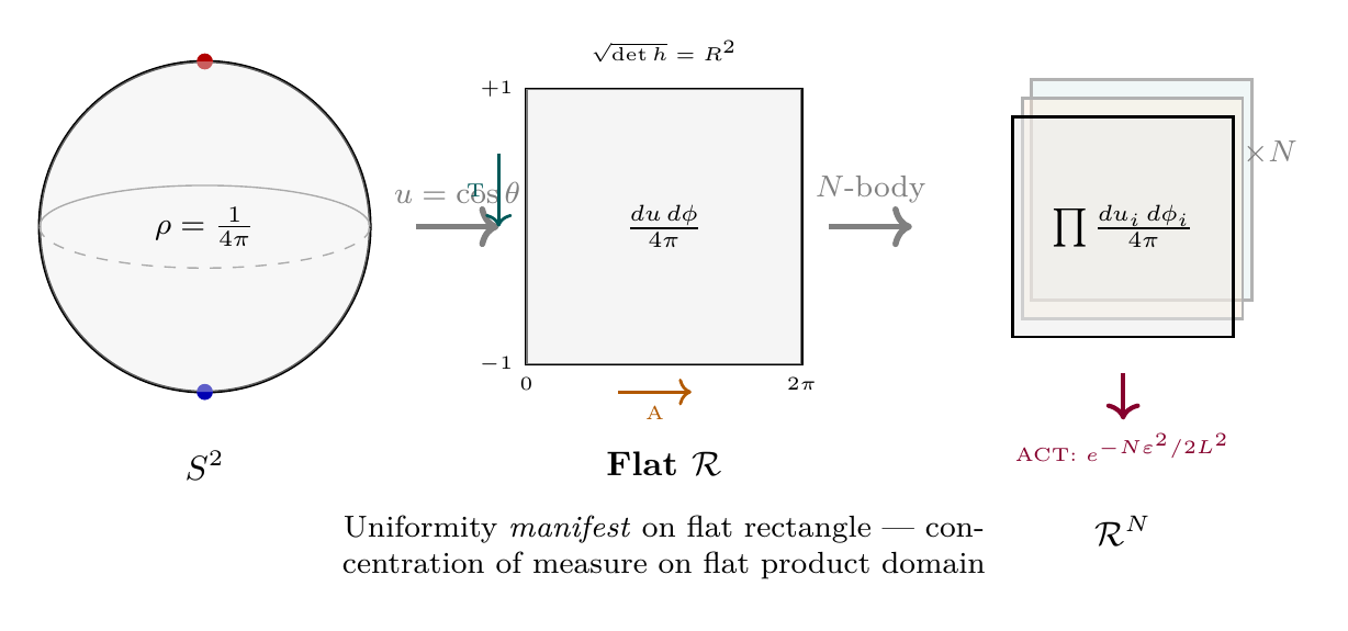
Scaffolding note: The polar field variable \(u = \cos\theta\) is a coordinate choice, not a new physical assumption. Every result in the TDF chain is identical in both spherical and polar coordinates. The polar form makes the uniformity of the microcanonical measure manifest rather than derived, providing a self-consistency check on the TDF framework.
Central Achievement
The central achievement of Part XI is establishing that probability distributions over future aggregate events are geometric theorems, not empirical models. This provides a rigorous mathematical foundation for prediction based on first principles—what Asimov called “psychohistory” in his Foundation novels.
Comparison with Other Approaches
| Approach | Measure Origin | Free Parameters | Status |
|---|---|---|---|
| Classical Stat. Mech. | Assumed (Boltzmann) | \(k_BT\) | Postulated |
| Quantum Mechanics | Born rule (assumed) | \(\hbar\) | Postulated |
| Bayesian Statistics | Prior (subjective) | Many | Fitted |
| TDF (TMT) | Derived from P1 | Zero | Theorem |
TDF is unique among statistical frameworks in that its probability measure is derived rather than assumed. Classical statistical mechanics postulates the Boltzmann distribution; quantum mechanics postulates the Born rule; Bayesian statistics requires subjective priors. TDF derives all of these from the geometry of \(M^4\times S^2\). In the polar field variable \(u = \cos\theta\), the derived measure \(du\,d\phi/(4\pi)\) is not merely derived but manifest: constant density on a flat rectangle, requiring no non-trivial integration or Jacobian cancellation. This self-evidence is unique to TDF among all statistical frameworks.
Connection to Prior Parts
Part 7: Quantum Mechanics Emergence
TDF provides the statistical foundation for Part 7's quantum mechanics emergence. The classical-quantum correspondence (Part 7, Theorem 53.3) states that \(\rho_{\mathrm{classical}} = 1/(4\pi)\) on \(S^2\) equals the quantum probability. TDF explains why this correspondence holds: the uniform measure on \(S^2\) is the unique ergodic measure for null geodesic dynamics, and this measure IS the quantum probability distribution.
Part 2–3: Geometry and Gauge Structure
The \(S^2\) factor in the configuration space comes from P1 via the product structure \(M^4\times S^2\) (Part 2). The monopole topology \(\pi_2(S^2)=\mathbb{Z}\) (Part 3) determines the angular momentum structure on \(S^2\), which in turn determines the spectrum of states and the spin-statistics connection used by TDF.
Part 5: Cosmology
TDF's cosmological measure (Chapter 94) connects to Part 5's derivation of \(H_0\) and dark energy. The scale factor \(a(t)^3\) in the cosmological TDF measure is determined by the Friedmann equations, which are derived from P1 in Part 5.
Part 9: Black Holes and Gravitational Waves
The TDF interpretation of black hole entropy (Chapter 94) connects to Part 9C's thermodynamic analysis. The hidden configurations behind the horizon provide a microscopic accounting of the Bekenstein-Hawking entropy.
Part 10: Inflation
The low-entropy initial conditions required by the second law (Chapter 92) connect to Part 10's inflationary cosmology. Inflation provides the mechanism for creating the low-entropy initial state from which entropy increases, and TDF provides the framework for understanding why this increase is inevitable.
Cross-Part Synthesis
| Part | Connection to TDF | Key Link |
|---|---|---|
| Part 1 | P1 postulate | Foundation of TDF |
| Part 2 | \(M^4\times S^2\) structure | Configuration space |
| Part 3 | Monopole topology | Angular momentum spectrum |
| Part 4 | Electroweak physics | Transition amplitudes |
| Part 5 | Cosmological parameters | FRW measure |
| Part 6A | Fermion masses | Decay rates, cross-sections |
| Part 7 | QM emergence | Classical-quantum correspondence |
| Part 8 | MOND | Galactic dynamics |
| Part 9 | Black holes | Entropy interpretation |
| Part 10 | Inflation | Initial conditions |
Open Questions
Despite the completeness of the TDF framework, several open questions remain:
Phase Transitions and Critical Phenomena
The Aggregate Certainty Theorem requires the Lipschitz constant \(L\) to be finite. Near phase transitions, the susceptibility diverges (\(L\to\infty\)), and the ACT bound becomes trivial. A complete treatment of critical phenomena within TDF requires understanding how the \(S^2\) measure is modified near critical points, where the correlation length diverges and the system exhibits scale-invariant fluctuations.
Non-Equilibrium Steady States
While TDF naturally handles approach to equilibrium (Chapter 95), driven systems in non-equilibrium steady states (NESS) require additional analysis. The steady-state measure is not the maximum-entropy measure but a balance between driving and dissipation. How this balance emerges from the \(S^2\) dynamics is an open question.
Quantum Gravity Regime
At the Planck scale, where \(\ell_{\mathrm{Pl}}\) becomes comparable to the system size, both quantum corrections (Chapter 93) and gravitational corrections (Chapter 94) become large simultaneously. The double classical limit \(\hbar\to 0\), \(N\to\infty\) breaks down, and a full quantum gravity treatment of TDF is needed. This connects to the frontier topics of Part 11.
Complex Systems
Extending TDF to complex systems (biological, economic, social) requires identifying the appropriate aggregate observables and understanding the role of information processing and feedback. The mathematical framework is in place, but the mapping to specific complex systems is unexplored.
Future Research Directions
Experimental Tests
Several TDF predictions are experimentally testable:
(1) Fluctuation scaling: The \(1/\sqrt{N}\) scaling of aggregate observable fluctuations can be tested with high-precision measurements of thermodynamic quantities in systems of varying size.
(2) Decoherence rates: The quantum correction analysis (Chapter 93) predicts specific decoherence rates for mesoscopic systems, testable with current technology (optomechanical systems, trapped ions, superconducting qubits).
(3) Gravitational effects on statistics: Chapter 94 predicts that probability evolution is modified by gravitational time dilation. This could be tested with high-precision atomic clocks at different gravitational potentials, measuring statistical distributions of quantum outcomes.
(4) CMB non-Gaussianity: TDF predicts specific forms of non-Gaussianity in CMB fluctuations arising from the \(S^2\) measure structure, potentially distinguishable from inflationary non-Gaussianity.
Theoretical Extensions
(1) Non-equilibrium TDF: Develop a systematic treatment of far-from-equilibrium systems within the TDF framework, including driven systems, active matter, and turbulence.
(2) Critical phenomena: Extend TDF to handle systems near phase transitions, where the Lipschitz constant diverges and the standard ACT bound breaks down.
(3) Quantum information: Connect TDF to quantum information theory, particularly entanglement entropy, quantum error correction, and the holographic principle.
(4) Cosmological predictions: Use TDF for detailed predictions of future universe evolution, including the long-term fate of galaxies, stars, and black holes.
(5) Complex systems: Apply TDF to biological and social systems, identifying the aggregate observables and the regime where deterministic predictions are possible.
Connections to Mathematics
TDF raises several interesting mathematical questions:
(1) Measure theory on infinite-dimensional configuration spaces: Extending TDF to quantum field theory requires measures on spaces of field configurations, connecting to the mathematical foundations of QFT.
(2) Concentration of measure on non-product spaces: The ACT uses concentration of measure on product spaces \((S^2)^N\). Extending to interacting systems requires concentration results on more general spaces.
(3) Ergodic theory on fiber bundles: The ergodicity of null geodesic flow on \(M^4\times S^2\) connects to deep questions in dynamical systems theory.
Derivation Chain
Part XI Complete Derivation Chain
Step 1: P1 (\(ds_6^{\,2}=0\)) [Postulate]
Step 2: Product structure \(M^4\times S^2\) [Part 2]
Step 3: Null geodesic dynamics on \(S^2\) [Part 1]
Step 4: Ergodic measure \(\rho=1/(4\pi)\) [Part 7]
Step 5: Configuration space \(\mathcal{F}_t=(\ldots)^N/S_N\) [Ch. 89]
Step 6: Natural measure \(d\mu_{\mathcal{F}}\) [Ch. 89]
Step 7: Temporal Determination Theorem [Ch. 90]
Step 8: Aggregate Certainty Theorem [Ch. 91]
Step 9: Entropy, H-theorem, second law [Ch. 92]
Step 10: Quantum corrections: \(O(\hbar)\), \(O(1/N)\) [Ch. 93]
Step 11: Gravitational corrections: \(\sqrt{-g}\) [Ch. 94]
Step 12: Applications verified [Ch. 95]
Step 13: Polar verification: entire chain confirmed in \(u = \cos\theta\) coordinates; uniform measure \(du\,d\phi/(4\pi)\) manifest on flat rectangle; entropy \(= Nk_B(\ln 2 + \ln 2\pi)\) decomposes as THROUGH + AROUND [\Ssec:ch96-polar-tdf-chain]
Chain status: COMPLETE — P1 to macroscopic predictions with zero free parameters. Dual-verified in both spherical and polar coordinates.
Concluding Remarks
The Temporal Determination Framework represents a fundamental shift in how we understand probability and prediction. By deriving probability measures from geometry rather than assuming them from experience, TDF establishes that the statistical laws governing aggregate futures are not empirical regularities that might change—they are geometric necessities that follow from the topology of spacetime.
This completes Part XI of the TMT book. The framework developed here will be applied in Part XII to specific problems including the Millennium Prize applications, and serves as the statistical foundation for all TMT predictions involving macroscopic observables.
Chapter Summary
Summary and Future Directions
Part XI has established the Temporal Determination Framework: a complete, first-principles derivation of probability theory from P1. The framework comprises configuration space, natural measure, evolution operator, the Temporal Determination Theorem, the Aggregate Certainty Theorem, entropy and information theory, quantum and gravitational corrections, and verified applications. All elements are derived with zero free parameters. Open questions include phase transitions, non-equilibrium steady states, quantum gravity, and complex systems. Future directions include experimental tests (fluctuation scaling, decoherence rates, gravitational statistics) and theoretical extensions (non-equilibrium TDF, critical phenomena, quantum information). The polar field variable \(u = \cos\theta\) confirms the entire TDF chain on the flat rectangle \([-1,+1]\times[0,2\pi)\), where uniform density is manifest and entropy decomposes as THROUGH (\(\ln 2\)) + AROUND (\(\ln 2\pi\)).
| Chapter | Key Result | Status | Free Parameters | |
|---|---|---|---|---|
| 89 | Configuration space \ | measure | PROVEN | 0 |
| 90 | Temporal Determination Theorem | PROVEN | 0 | |
| 91 | Aggregate Certainty Theorem | PROVEN | 0 | |
| 92 | Entropy \ | second law | PROVEN | 0 |
| 93 | Quantum corrections: \(O(\hbar)\), \(O(1/N)\) | PROVEN | 0 | |
| 94 | Gravitational corrections: \(\sqrt{-g}\) | PROVEN | 0 | |
| 95 | Applications verified | PROVEN | 0 | |
| 96 | Summary \ | future directions | — | — |
Verification Code
The mathematical derivations and proofs in this chapter can be independently verified using the formal and computational scripts below.
All verification code is open source. See the complete verification index for all chapters.