Chern-Simons Theory, Quantum Groups, and Topological Closure
The 2-sphere admits a single quantum state. This is not a choice — it is the topological rigidity of \(S^2\) asserting itself at every level of mathematical structure.
Chapter Overview
The preceding chapters of Part XIV established the arithmetic infrastructure of TMT: the motive (Chapter 162), modular forms (Chapter 163), \(L\)-functions (Chapter 164), Arakelov geometry (Chapter 165), period duality (Chapter 166), and class field theory (Chapter 167). These developments revealed that every integer, every prime, and every algebraic structure appearing in TMT is uniquely determined by the geometry of \(S^2 \cong \mathbb{P}^1\).
This chapter completes the topological side of the argument. We prove that TMT, viewed through the lens of topological quantum field theory and quantum groups, is uniquely determined at every level of structure — classical, quantum, and categorical. The key results are:
- The 2-sphere state space is 1-dimensional: \(\dim Z(S^2) = 1\) (unique vacuum).
- Chern–Simons theory at level \(k = 12\) with gauge group \(\SU(2)\) is the unique TQFT compatible with the TMT structure.
- The quantum group \(U_q(\mathfrak{su}_2)\) at \(q = e^{2\pi i/14}\) — a root of unity forced by \(k = 12\) — provides the algebraic backbone.
- The deformation parameter \(q\) is fixed, not free: since \(\mathrm{HH}^2(\mathbb{P}^1) = 0\) (Chapter 161), no deformations of the TMT structure exist.
- The modular tensor category \(\mathrm{Rep}(\SU(2)_{12})\), with its 13 simple objects and rigid fusion rules, uniquely determines the 3-dimensional TQFT via the Reshetikhin–Turaev construction.
The derivation chain for this chapter runs:
Topological Quantum Field Theory: Axioms and Classification
We begin with the mathematical framework that will govern the entire chapter: the axioms of topological quantum field theory as formulated by Atiyah and Segal.
The Atiyah–Segal Axioms
The symmetric monoidal category \(\mathrm{Cob}_d\) has:
- Objects: Closed oriented smooth \((d-1)\)-manifolds \(\Sigma\).
- Morphisms: Diffeomorphism classes of compact oriented smooth \(d\)-manifolds \(M\) with \(\partial M = \overline{\Sigma}_1 \sqcup \Sigma_2\) (cobordisms from \(\Sigma_1\) to \(\Sigma_2\)).
- Composition: Gluing along common boundary: if \(M_1: \Sigma_1 \to \Sigma_2\) and \(M_2: \Sigma_2 \to \Sigma_3\), then \(M_2 \circ M_1 = M_2 \cup_{\Sigma_2} M_1: \Sigma_1 \to \Sigma_3\).
- Identity: The cylinder \(\Sigma \times [0,1]: \Sigma \to \Sigma\).
- Monoidal structure: Disjoint union \(\sqcup\) with unit \(\emptyset\).
A \(d\)-dimensional TQFT is a symmetric monoidal functor:
- To each closed \((d-1)\)-manifold \(\Sigma\): a finite-dimensional vector space \(Z(\Sigma)\).
- To each cobordism \(M: \Sigma_1 \to \Sigma_2\): a linear map \(Z(M): Z(\Sigma_1) \to Z(\Sigma_2)\).
- To each closed \(d\)-manifold \(M\): a complex number \(Z(M) \in \mathbb{C}\) (the partition function).
A TQFT \(Z: \mathrm{Cob}_d \to \mathrm{Vect}\) satisfies the following axioms:
- Functoriality: \(Z(M_2 \circ M_1) = Z(M_2) \circ Z(M_1)\) for composable cobordisms.
- Monoidal: \(Z(\Sigma_1 \sqcup \Sigma_2) = Z(\Sigma_1) \otimes Z(\Sigma_2)\).
- Unit: \(Z(\emptyset) = \mathbb{C}\).
- Duality: \(Z(\overline{\Sigma}) = Z(\Sigma)^*\) (orientation reversal gives dual space).
- Identity: \(Z(\Sigma \times [0,1]) = \mathrm{id}_{Z(\Sigma)}\) (cylinder gives identity map).
These follow directly from the symmetric monoidal functor structure. Functoriality is the functor axiom. The monoidal axiom encodes \(Z(\Sigma_1 \sqcup \Sigma_2) \cong Z(\Sigma_1) \otimes Z(\Sigma_2)\) via the monoidal structure. The unit axiom \(Z(\emptyset) = \mathbb{C}\) follows from the empty manifold being the monoidal unit. Duality comes from the orientation-reversal involution on \(\mathrm{Cob}_d\). The identity axiom follows from the cylinder being the identity morphism in \(\mathrm{Cob}_d\). □ □
For TMT, the relevant dimensions are:
| \(d\) | Objects | Morphisms | Physical theory | TMT relevance |
|---|---|---|---|---|
| 2 | \(S^1\) | Surfaces | 2D CFT | \(S^2\) as 2-manifold |
| 3 | \(\Sigma_g\) (genus \(g\)) | 3-manifolds | Chern–Simons | TMT-TQFT |
Each TQFT axiom is compatible with the TMT structure:
- Functoriality: The constraint \(ds_6^2 = 0\) is preserved under composition of cobordisms because it is a local condition on the metric. Temporal evolution operators compose.
- Monoidal: For disjoint interfaces \(S^2_1 \sqcup S^2_2\), locality of the \(ds_6^2 = 0\) constraint gives \(Z(S^2_1 \sqcup S^2_2) = Z(S^2_1) \otimes Z(S^2_2)\).
- Duality: Orientation reversal of \(S^2\) exchanges the “inside” and “outside” of the interface, corresponding to CPT conjugation of the 4D physics. This gives \(Z(\overline{S^2}) = Z(S^2)^*\).
2D TQFT Classification
Two-dimensional topological quantum field theories are classified by commutative Frobenius algebras. Specifically, there is an equivalence of categories:
The classification proceeds by pair-of-pants decomposition of surfaces. Every closed oriented surface \(\Sigma_g\) of genus \(g\) decomposes into pairs of pants (the multiplication) and caps (the trace). The TQFT axioms force \(Z(S^1)\) to carry both a multiplication \(\mu: Z(S^1) \otimes Z(S^1) \to Z(S^1)\) and a trace \(\varepsilon: Z(S^1) \to \mathbb{C}\) making it a commutative Frobenius algebra. The partition function on genus-\(g\) surfaces is:
TMT is not a 2D TQFT (it has time evolution and the 6D scaffolding suggests higher structure), but it possesses a 2D shadow: the restriction to \(S^2\) slices yields a Frobenius algebra with trace determined by the monopole integral:
The \(S^2\) State Space: \(\dim Z(S^2) = 1\)
The most fundamental result connecting TMT to TQFT is the uniqueness of the vacuum on \(S^2\).
\(S^2\) bounds the 3-ball \(B^3\). By the TQFT axioms, the cobordism \(B^3: \emptyset \to S^2\) provides a linear map \(Z(B^3): \mathbb{C} \to Z(S^2)\), hence a vector \(v = Z(B^3)(1) \in Z(S^2)\). Since \(B^3\) is the unique filling of \(S^2\) (up to diffeomorphism), and since \(\pi_1(S^2) = 0\) gives a trivial representation variety \(\mathrm{Hom}(\pi_1(S^2), G)/G = \text{pt}\), the state space is 1-dimensional:
TMT also has a unique vacuum on \(S^2\): the constraint \(ds_6^2 = 0\) on \(M^4 \times S^2\) determines a unique classical ground state on the interface. The coincidence \(\dim Z(S^2) = 1\) in both TQFT and TMT is not accidental — it reflects the topological rigidity of \(S^2\). The trivial fundamental group \(\pi_1(S^2) = 0\) means there are no non-contractible Wilson loops on \(S^2\) itself, consistent with the simply-connected gauge group \(\SU(2)\).
For \(\SU(2)\) Chern–Simons at level \(k\), the state space dimensions on standard surfaces are:
For \(S^2\): proved in Theorem thm:168-dim-ZS2. For \(T^2\): the torus has \(\pi_1(T^2) = \mathbb{Z}^2\), and the state space is spanned by integrable highest-weight representations of the affine Lie algebra \(\widehat{\mathfrak{su}(2)}_k\). There are exactly \(k+1\) such representations (spins \(j = 0, \frac{1}{2}, \ldots, \frac{k}{2}\)). The general formula follows from the Verlinde formula, which computes the dimension of the space of conformal blocks of the WZW model on \(\Sigma_g\). □ □
At \(k = 12\): \(\dim Z(T^2) = 13\), giving 13 integrable representations — connecting directly to the categorical prime 13 identified in Chapter 160.
Chern–Simons at Level 12
The Chern–Simons Action
For a compact Lie group \(G\) and connection \(A\) on a 3-manifold \(M\), the Chern–Simons action is:
Chern–Simons theory defines a 3-dimensional TQFT:
- \(Z(\Sigma)\) = space of conformal blocks of the WZW (Wess–Zumino–Witten) model on \(\Sigma\).
- \(Z(M)\) = topological invariant of the 3-manifold \(M\), related to quantum group data.
- Wilson lines in representation \(R\) along knots \(K\) give the Jones polynomial: \(\langle W_R(K) \rangle = J_R(K; q)\).
Five Arguments for \(k = 12\)
The Chern–Simons level compatible with the TMT structure is uniquely \(k = 12\), selected by five independent arguments:
- Product structure: \(k = n_g \times n_H = 3 \times 4 = 12\), the product of the generation number and the Higgs multiplicity, both derived from the \(S^2\) geometry (Chapter 160).
- Bernoulli denominator: \(k = 12\) is the smallest index such that all five primes satisfying \((p-1) \mid k\) contribute to \(\mathrm{denom}(B_{12}) = 2730 = 2 \cdot 3 \cdot 5 \cdot 7 \cdot 13\) (Chapter 163).
- Dimension lcm: \(k = \mathrm{lcm}(\dim_{\mathbb{R}}(M^4), \dim_{\mathbb{R}}(M^4 \times S^2)) = \mathrm{lcm}(4, 6) = 12\).
- Central charge: \(c = 3k/(k+2) = 36/14 = 18/7\) involves only TMT primes in the denominator.
- Modular invariance: The modular \(S\)-matrix at \(k = 12\) has entries involving \(\sin(n\pi/14)\), with the TMT prime 7 controlling the angular resolution.
No other small value of \(k\) satisfies all five criteria simultaneously.
Arguments (1)–(5) are proved in Chapters 160, 163, and the master Part 15C analysis. The uniqueness follows by elimination: \(k = 6\) gives \(c = 9/4\) (no prime 7), \(k = 4\) gives \(c = 2\) (integer, no prime structure), \(k = 24\) gives \(c = 36/13\) (denominator 13, categorical not arithmetic). Combined with the deformation rigidity \(\mathrm{HH}^2(\mathbb{P}^1) = 0\) (Chapter 161), no alternative level exists. □ □
The Central Charge and Quantum Parameter
The modular \(S\)-matrix at \(k = 12\) is a \(13 \times 13\) matrix with entries:
The fusion coefficients of \(\SU(2)\) at level \(k\) are:
Quantum Groups: \(U_q(\mathfrak{su}_2)\) at the Root of Unity \(q = e^{2\pi i/14}\)
The algebraic backbone of Chern–Simons theory at level \(k = 12\) is the quantum group \(U_q(\mathfrak{su}_2)\) at the root of unity \(q = e^{2\pi i/14}\). This section develops the Hopf algebra structure from scratch.
Definition and Relations
The quantum group \(U_q(\mathfrak{su}_2)\) is the Hopf algebra over \(\mathbb{C}(q)\) generated by \(E, F, K, K^{-1}\) with relations:
Hopf Algebra Structure
\(U_q(\mathfrak{su}_2)\) is a Hopf algebra with:
- Coproduct (how charges combine):
- Counit: \(\varepsilon(K) = 1\), \(\varepsilon(E) = \varepsilon(F) = 0\).
- Antipode: \(S(K) = K^{-1}\), \(S(E) = -EK^{-1}\), \(S(F) = -KF\).
The coproduct \(\Delta\) encodes how gauge charges combine in tensor products — the quantum analog of the Clebsch–Gordan decomposition.
One verifies the Hopf algebra axioms directly: the coproduct is an algebra homomorphism \(\Delta: U_q \to U_q \otimes U_q\), the counit satisfies \((\varepsilon \otimes \mathrm{id}) \circ \Delta = \mathrm{id}\), and the antipode satisfies \(\mu \circ (S \otimes \mathrm{id}) \circ \Delta = \eta \circ \varepsilon\) (where \(\mu\) is multiplication and \(\eta\) is the unit). All verifications reduce to the defining relations eq:168-quantum-relations. □ □
Representation Theory at Root of Unity: 13 Integrable Representations
At the root of unity \(q = e^{2\pi i/14}\), the representation theory of \(U_q(\mathfrak{su}_2)\) undergoes a dramatic truncation.
Generic \(q\) vs. Root of Unity
For generic \(q\) (not a root of unity), the representation theory of \(U_q(\mathfrak{su}_2)\) mirrors the classical case:
- Irreducible finite-dimensional representations \(V_j\) for each \(j \in \frac{1}{2}\mathbb{Z}_{\geq 0}\) (spin \(j = 0, \frac{1}{2}, 1, \frac{3}{2}, \ldots\)).
- Each \(V_j\) has dimension \(\dim(V_j) = 2j + 1\) (same as classical \(\SU(2)\)).
- Tensor product rules are deformed but combinatorially similar to the classical Clebsch–Gordan rules.
At \(q = e^{2\pi i/(k+2)}\) (the \((k+2)\)th root of unity):
- Only finitely many irreducible representations survive: spins \(j = 0, \frac{1}{2}, 1, \ldots, \frac{k}{2}\).
- The total number of integrable representations is \(k + 1\).
- The tensor product becomes the truncated tensor product: spins exceeding \(k/2\) are projected out.
- The truncated representation category forms a modular tensor category.
At \(k = 12\) (so \(q = e^{2\pi i/14}\)):
At a root of unity \(q = e^{2\pi i/(k+2)}\), the quantum dimension \([2j+1]_q = \sin((2j+1)\pi/(k+2))/\sin(\pi/(k+2))\) vanishes for \(j = (k+2)/2\), and representations with \(j > k/2\) have zero or negative quantum dimension. The consistent truncation retains only \(j \in \{0, \frac{1}{2}, \ldots, \frac{k}{2}\}\), giving \(k+1\) representations. At \(k = 12\): \(k+1 = 13\). □ □
Quantum Integers
Quantum integers satisfy:
- Classical limit: \([n]_q \to n\) as \(q \to 1\).
- Symmetry: \([n]_q = [n]_{q^{-1}}\).
- Recursion: \([n+1]_q = q[n]_q + q^{-n}\).
- Periodicity at roots of unity: \([k+2]_q = 0\), so \([14]_q = 0\) at \(k = 12\).
- Quantum dimension: The quantum dimension of the spin-\(j\) representation is \(d_j = [2j+1]_q\).
At \(q = e^{i\pi/7}\), the quantum integer \([2]_q\) is:
The Modular Tensor Category and Reshetikhin–Turaev
The 13 integrable representations of \(U_q(\mathfrak{su}_2)\) at \(q = e^{2\pi i/14}\) organize into a mathematical structure of remarkable rigidity: a modular tensor category.
Modular Tensor Categories
A modular tensor category (MTC) is a ribbon fusion category \(\mathcal{C}\) over \(\mathbb{C}\) such that:
- \(\mathcal{C}\) has finitely many isomorphism classes of simple objects \(\{V_0 = \mathbf{1}, V_1, \ldots, V_r\}\).
- \(\mathcal{C}\) has a braiding \(c_{V,W}: V \otimes W \xrightarrow{\sim} W \otimes V\) and a twist \(\theta_V: V \xrightarrow{\sim} V\) (ribbon structure).
- The \(S\)-matrix \(S_{ij} = \mathrm{tr}(c_{V_j, V_i} \circ c_{V_i, V_j})\) is invertible (the modularity condition).
- The fusion rules \(V_i \otimes V_j \cong \bigoplus_k N_{ij}^k V_k\) have non-negative integer coefficients.
The category \(\mathrm{Rep}(\SU(2)_{12})\) of integrable representations of \(\SU(2)\) at level 12 forms a modular tensor category with:
- 13 simple objects: \(V_0, V_1, \ldots, V_{12}\) (spins \(j = 0, \frac{1}{2}, \ldots, 6\)).
- Fusion rules: \(V_i \otimes V_j = \bigoplus_{m=|i-j|}^{\min(i+j, \, 2k - i - j)} V_m\) (truncated Clebsch–Gordan).
- Braiding: Determined by the \(R\)-matrix of \(U_q(\mathfrak{su}_2)\) at \(q = e^{i\pi/7}\).
- Modular \(S\)-matrix: The \(13 \times 13\) matrix eq:168-s-matrix is invertible (its determinant is non-zero, confirming modularity).
The category \(\mathrm{Rep}(U_q(\mathfrak{su}_2))\) at a root of unity \(q = e^{2\pi i/(k+2)}\) is a well-studied example of a modular tensor category. The fusion rules follow from the truncated tensor product (Theorem thm:168-root-of-unity). The \(R\)-matrix of \(U_q(\mathfrak{su}_2)\) provides the braiding, and the ribbon element gives the twist. Modularity (invertibility of \(S\)) follows from the Verlinde formula: \(S\) diagonalizes the fusion rules, and all quantum dimensions \(d_j > 0\) for \(0 \leq j \leq k\). At \(k = 12\), all 13 quantum dimensions are positive, confirming the non-degeneracy of \(S\). □ □
The Reshetikhin–Turaev Construction
Every modular tensor category \(\mathcal{C}\) uniquely determines a 3-dimensional TQFT via the Reshetikhin–Turaev construction:
The Reshetikhin–Turaev construction proceeds as follows: given a closed 3-manifold \(M\), represent \(M\) as surgery on a framed link \(L\) in \(S^3\). The partition function is:
Since the TMT structure determines:
- The gauge group \(\SU(2)\) (from \(\mathrm{Iso}(S^2)\) — Chapter 3),
- The level \(k = 12\) (five independent arguments — Theorem thm:168-k-equals-12),
- The quantum group \(U_q(\mathfrak{su}_2)\) at \(q = e^{i\pi/7}\),
- The modular tensor category \(\mathrm{Rep}(\SU(2)_{12})\),
the Reshetikhin–Turaev theorem guarantees that this data uniquely determines a 3-dimensional TQFT. There is no freedom: the TQFT is as unique as the 2-sphere itself.
The Deformation Parameter Is Fixed: No Quantum Alternatives
The quantum group \(U_q(\mathfrak{su}_2)\) at \(q = e^{i\pi/7}\) is the algebraic backbone of Chern–Simons theory at level \(k = 12\). A natural question arises: could \(q\) take a different value? Could the TMT framework accommodate a deformation, producing a family of theories indexed by \(q\)? The answer is no—and the proof is cohomological.
Hochschild Cohomology and Deformation Rigidity
For an associative algebra \(\mathcal{A}\) over a field \(k\), the Hochschild cohomology \(\mathrm{HH}^n(\mathcal{A}, \mathcal{A})\) controls the deformation theory of \(\mathcal{A}\):
- \(\mathrm{HH}^0(\mathcal{A}, \mathcal{A})\): centre of \(\mathcal{A}\),
- \(\mathrm{HH}^1(\mathcal{A}, \mathcal{A})\): outer derivations (infinitesimal automorphisms),
- \(\mathrm{HH}^2(\mathcal{A}, \mathcal{A})\): first-order deformations,
- \(\mathrm{HH}^3(\mathcal{A}, \mathcal{A})\): obstructions to extending deformations.
A vanishing \(\mathrm{HH}^2(\mathcal{A}, \mathcal{A}) = 0\) means every infinitesimal deformation is trivial—the algebra is rigid.
The Hochschild cohomology of the structure sheaf of \(\mathbb{P}^1 = S^2\) satisfies:
By the Hochschild–Kostant–Rosenberg theorem for smooth varieties, \(\mathrm{HH}^n(X) \cong \bigoplus_{p+q=n} H^q(X, \bigwedge^p T_X)\). For \(X = \mathbb{P}^1\):
Since \(\mathrm{HH}^2(\mathbb{P}^1) = 0\), the TMT interface \(S^2 \cong \mathbb{P}^1\) is rigid. The quantum group parameter \(q = e^{i\pi/7}\) is not a free parameter that could be varied—it is the unique value forced by:
- \(k = 12\) (five independent arguments — Theorem thm:168-k-equals-12),
- \(q = e^{2\pi i/(k+2)} = e^{2\pi i/14} = e^{i\pi/7}\) (root of unity for level \(k\)).
No continuous family of TMT-like theories exists. The deformation is not merely preferred—it is unique.
The rigidity result \(\mathrm{HH}^2(\mathbb{P}^1) = 0\) has a direct physical interpretation within the TMT framework:
- From 4D: The extra-dimensional interface \(S^2\) is rigid—its complex structure cannot be deformed. The modulus \(R_0\) controls the scale but the shape is locked.
- From 3D: The \(S^2\) fibres in the Kaluza–Klein reduction cannot be “squashed” or deformed into a different topology. The round metric is the unique Einstein metric on \(S^2\) (up to scale).
This dual perspective confirms that the quantum parameter \(q = e^{i\pi/7}\) is as rigid as the 2-sphere itself. There is no “almost-TMT” with \(q = e^{i\pi/7} + \epsilon\).
Wilson Lines as Monopole Harmonics
In Chern–Simons theory, Wilson lines are the fundamental observables. In TMT, monopole harmonics are the fundamental fields on \(S^2\). We now establish that these two descriptions coincide.
Wilson Lines in Chern–Simons Theory
This is Witten's foundational result. The Chern–Simons path integral with Wilson line insertion defines a topological invariant because the CS action is metric-independent. The Reshetikhin–Turaev construction provides a rigorous combinatorial definition: represent \(K\) as a braid closure, apply the \(R\)-matrix of \(U_q(\mathfrak{su}_2)\) at each crossing, and take the quantum trace. The result is independent of the braid representative by the Markov theorem. □ □
The Monopole–Wilson Correspondence
In the TMT framework at level \(k = 12\), there is a precise correspondence between monopole harmonics on \(S^2\) and Wilson lines in Chern–Simons theory:
| TMT (monopole) | CS (Wilson line) | Algebraic |
|---|---|---|
| Monopole charge \(j\) | Representation spin \(j\) | Weight \(j \in \{0, \tfrac{1}{2}, \ldots, 6\}\) |
| Monopole worldline on \(S^2\) | Curve \(\gamma \subset S^3\) | Knot in 3-manifold |
| Monopole harmonic \(Y^\ell_m\) | Wilson line \(W_j(\gamma)\) | Module over \(U_q(\mathfrak{su}_2)\) |
| Monopole fusion | Wilson line fusion | Truncated tensor product |
The expectation value of a Wilson line \(W_j(\gamma)\) in Chern–Simons at \(k = 12\) gives the monopole contribution:
The correspondence rests on three identifications:
- Charges match representations: TMT monopoles carry charges classified by \(\mathrm{Iso}(S^2) = \mathrm{SO}(3) \supset \mathrm{SU}(2)\), with allowed spins \(j \in \{0, \frac{1}{2}, 1, \ldots\}\). At level \(k = 12\), the truncation of Theorem thm:168-root-of-unity restricts to \(j \in \{0, \frac{1}{2}, \ldots, 6\}\)—exactly the 13 integrable representations. Wilson lines in these representations are the only allowed observables.
- Fusion rules agree: Monopole “fusion” (bringing two monopoles together) must obey the truncated tensor product:
- Path integrals coincide: The TMT path integral with a monopole insertion at a point \(p \in S^2\) and worldline \(\gamma\) reduces, in the topological sector, to the CS path integral with Wilson line insertion \(W_j(\gamma)\).
□ □
The truncated fusion rules at \(k = 12\) produce:
Jones Polynomial and Monopole Knot Invariants
The Jones Polynomial at \(q = e^{i\pi/7}\)
The Jones polynomial \(V_K(q)\) of a knot \(K\) is a knot invariant arising from the representation theory of \(U_q(\mathfrak{su}_2)\):
- The representation category \(\mathrm{Rep}(U_q(\mathfrak{su}_2))\) is a ribbon category,
- \(V_K(q) = \mathrm{tr}_q(R_K)\), where \(R_K\) is the \(R\)-matrix braid representation of \(K\),
- \(V_K(q)\) equals the Wilson loop expectation value \(\langle W_{\frac{1}{2}}(K) \rangle\) in Chern–Simons theory.
The Jones polynomial satisfies \(V_K(q) \in \mathbb{Z}[q^{\pm 1/2}]\) and \(V_{\mathrm{unknot}}(q) = 1\) for all \(q\).
At \(k = 12\), the quantum parameter is \(q = e^{i\pi/7}\), and the coloured Jones polynomial evaluates knots at this 14th root of unity. For the unknot in representation \(j\):
The unknot evaluation is immediate from the quantum dimension formula (Theorem thm:168-quantum-integers). The trefoil formula follows from the skein relation for the Jones polynomial applied to the standard 3-crossing diagram of \(3_1\). The cyclotomic field \(\mathbb{Q}(\zeta_{14}) = \mathbb{Q}(\zeta_7)\) has discriminant involving only the prime \(7\), and the full Jones values live in \(\mathbb{Z}[\zeta_{14}]\), whose ramification set \(\{2, 7\}\) is contained in the TMT arithmetic spectrum. □ □
Monopole Worldlines as Knots
In the TMT framework, monopole worldlines on \(S^2\) (or more precisely in the 3-dimensional space \(S^2 \times \mathbb{R}\)) can form knots and links. Their topological invariants are:
| Knot feature | Invariant | TMT meaning |
|---|---|---|
| Linking number | \(\mathrm{lk}(\gamma_1, \gamma_2) \in \mathbb{Z}\) | Monopole–monopole interaction |
| Writhe | \(w(\gamma) \in \mathbb{Z}\) | Monopole self-energy |
| Jones polynomial | \(V_K(e^{i\pi/7}) \in \mathbb{Q}(\zeta_{14})\) | Quantum corrections to monopole action |
For an unknotted monopole worldline, \(V_{\mathrm{unknot}}(e^{i\pi/7}) = 1\): there are no quantum corrections from knotting topology.
The Jones polynomial can be categorified: Khovanov homology \(\mathrm{Kh}(K)\) is a bigraded homology theory satisfying \(\chi_q(\mathrm{Kh}(K)) = V_K(q)\), where \(\chi_q\) is the graded Euler characteristic. This categorification is richer: \(\mathrm{Kh}(K)\) distinguishes knots with equal Jones polynomials. For TMT, Khovanov homology of monopole worldlines provides a categorified invariant that encodes strictly more topological information than the Jones polynomial alone. In four dimensions, monopole worldsheets generalise knots to surfaces, and the natural invariant is a surface analogue of Khovanov homology.
Factorization Algebras and Extended TQFT
Factorization Algebras: Costello–Gwilliam Framework
While TQFT functors encode global information (state spaces and partition functions), factorization algebras encode local information (point-wise observables and their products). The distinction is important for TMT because the coupling constants are determined by local integrals on \(S^2\) (overlap integrals like \(\int |Y|^4 \, d\Omega\)), not just topological invariants.
A factorization algebra \(\mathcal{F}\) on a manifold \(M\) assigns:
- to each open set \(U \subseteq M\): a cochain complex \(\mathcal{F}(U)\),
- to disjoint opens \(U_1, \ldots, U_n \subseteq V\): a multiplication map
satisfying locality and associativity axioms. The global sections \(\mathcal{F}(M)\) recover the partition function, while local sections encode the OPE (operator product expansion).
The observables of TMT on \(S^2\) form a factorization algebra \(\mathcal{F}_{\mathrm{TMT}}\) determined by:
- \(\mathcal{F}_{\mathrm{TMT}}(U) \cong\) observables constructed from the monopole field \(Y\) restricted to \(U \subset S^2\),
- the multiplication map encodes the product structure of monopole harmonics via Clebsch–Gordan coefficients:
- the global sections \(\mathcal{F}_{\mathrm{TMT}}(S^2) \cong \mathbb{C}[Y_{\ell m}] / (ds_6^2 = 0)\), the polynomial ring in monopole harmonics modulo the extra-dimensional metric constraint.
The key point is that TMT observables on open sets \(U \subset S^2\) are polynomial functions of the monopole field \(Y\) restricted to \(U\). The Clebsch–Gordan decomposition of products \(Y_{\ell_1 m_1} \cdot Y_{\ell_2 m_2}\) provides the factorization product—it is local (depends only on the overlap at points in \(U\)), associative (by associativity of the Clebsch–Gordan coupling), and satisfies the factorization axiom: for disjoint opens, the fields on each open are independent, so the tensor product multiplication is well-defined. The Chern–Simons sector contributes a topological factorization algebra whose global sections recover \(Z(S^2) = \mathbb{C}\). □ □
Extended TQFT and the Cobordism Hypothesis
Fully extended TQFTs \(\mathrm{Bord}_d \to \mathcal{C}\) are classified by fully dualizable objects in \(\mathcal{C}\).
TMT defines a once-extended 3-dimensional TQFT. The fully dualizable object classifying this extended TQFT is the modular tensor category \(\mathrm{Rep}(\mathrm{SU}(2)_{12})\). The extended TQFT assigns:
| Dimension | Geometric input | TMT output |
|---|---|---|
| 0 (point) | Point on \(S^2\) | Category \(\mathrm{Rep}(\mathrm{SU}(2)_{12})\) |
| 1 (curve) | Arc on \(S^2\) | Functor (representation of path algebra) |
| 2 (surface) | \(S^2\) itself | Vector space \(Z(S^2) = \mathbb{C}\) |
| 3 (3-manifold) | Cobordism bounding \(S^2\) | Complex number (partition function) |
The modular tensor category \(\mathrm{Rep}(\mathrm{SU}(2)_{12})\) is a well-known example of a fully dualizable object in the Morita 3-category of tensor categories. By the cobordism hypothesis (Theorem thm:168-cobordism-hypothesis), this fully dualizable object uniquely determines a once-extended 3D TQFT. The assignments follow from the general Reshetikhin–Turaev–Turaev–Viro construction:
- A point is assigned the MTC itself (the generating object),
- A 1-manifold (arc) is assigned the endomorphism category, which by modularity is a functor category,
- A surface \(\Sigma\) is assigned the vector space \(Z(\Sigma)\) computed by the Reshetikhin–Turaev TQFT. For \(S^2\): \(Z(S^2) = \mathbb{C}\) (Theorem thm:168-dim-zs2).
- A 3-manifold \(M\) is assigned \(Z(M) \in \mathbb{C}\).
The decategorification from the 13-object category \(\mathrm{Rep}(\mathrm{SU}(2)_{12})\) down to the 1-dimensional space \(Z(S^2) = \mathbb{C}\) “forgets” most categorical information, retaining only the partition function. The extended version preserves the full structure. □ □
TQFT Closure: Uniqueness at Every Level
We now assemble the results of this chapter into the central closure theorem: the quasi-topological structure of TMT is uniquely determined at every level—classical, quantum, and categorical—with no deformations possible.
The Quasi-Topological Structure
The TMT framework depends on the metric only through the modulus \(R_0\), which is fixed by modulus stabilisation (Chapter 117). Once \(R_0\) is fixed, TMT is topological: the partition function \(Z(M)\) depends only on the topology of \(M\), not on the choice of Riemannian metric.
The Chern–Simons action \(S_{\mathrm{CS}} = \frac{k}{4\pi} \int_M \mathrm{tr}(A \wedge dA + \frac{2}{3} A \wedge A \wedge A)\) is manifestly metric-independent—it is written entirely in terms of differential forms and the wedge product, with no metric tensor appearing. The TMT coupling constants (\(g^2 = 4/(3\pi)\), etc.) are determined by overlap integrals on \(S^2\) at radius \(R_0\). Once \(R_0\) is stabilised, these constants are fixed numbers. The only metric dependence is through \(R_0\), and modulus stabilisation removes this last degree of freedom. □ □
The TQFT Closure Theorem
The quasi-topological structure of TMT is uniquely determined by the triple \((\mathrm{SU}(2), \, k = 12, \, R_0)\). No deformations exist at any level:
- Classical level: The gauge group \(\mathrm{SU}(2) = \mathrm{Iso}^+(S^2)\) is forced by the \(S^2\) geometry (Chapter 3). No other gauge group is consistent.
- Quantum level: The Chern–Simons level \(k = 12\) is determined by five independent arguments (Theorem thm:168-k-equals-12). The quantum parameter \(q = e^{i\pi/7}\) is locked (Corollary cor:168-q-locked).
- Categorical level: The modular tensor category \(\mathrm{Rep}(\mathrm{SU}(2)_{12})\) is rigid (13 simple objects with fixed fusion rules), and \(\mathrm{HH}^2(\mathbb{P}^1) = 0\) forbids deformations of the underlying geometry (Theorem thm:168-hh2-vanishing).
- Extended level: By the cobordism hypothesis, the once-extended 3D TQFT is uniquely classified by the fully dualizable object \(\mathrm{Rep}(\mathrm{SU}(2)_{12})\) (Theorem thm:168-tmt-extended).
At every level of mathematical description—classical, quantum, and categorical—the TMT topological structure admits no alternatives.
We verify each level:
- Classical: \(\mathrm{Iso}^+(S^2) = \mathrm{SO}(3)\), with double cover \(\mathrm{SU}(2)\). This is forced by the postulate \(P^1\) identifying \(S^2\) as the extra-dimensional interface.
- Quantum: The five arguments for \(k = 12\) (product structure, Bernoulli number, dimension lcm, central charge, modular invariance) independently select the same level. The quantum parameter \(q = e^{2\pi i/(k+2)} = e^{i\pi/7}\) is then determined. Theorem thm:168-hh2-vanishing (\(\mathrm{HH}^2(\mathbb{P}^1) = 0\)) ensures no continuous deformation family exists.
- Categorical: A modular tensor category is a rigid algebraic structure: the fusion rules, braiding, and twist are determined by the choice of quantum group and level. Given \(\mathrm{SU}(2)\) and \(k = 12\), the MTC \(\mathrm{Rep}(\mathrm{SU}(2)_{12})\) is uniquely determined (up to equivalence) by the Reshetikhin–Turaev construction (Theorem thm:168-reshetikhin-turaev).
- Extended: The cobordism hypothesis gives a bijection between fully extended 3D TQFTs and fully dualizable objects. Since \(\mathrm{Rep}(\mathrm{SU}(2)_{12})\) is the unique MTC from the data above, the extended TQFT is unique.
Combining all four levels: the TMT topological sector is completely determined with zero free parameters beyond \(P^1\) and \(R_0\). □ □
The TQFT Closure Theorem (Theorem thm:168-tqft-closure) is one of the strongest rigidity results in the TMT programme. In most physical theories, the topological sector admits continuous families of parameters (e.g., the theta angle in QCD). TMT's topological sector is completely rigid: the gauge group, level, quantum parameter, MTC, and extended TQFT are all uniquely determined. This is the mathematical reflection of the physical principle that TMT has no free parameters beyond the single postulate \(P^1\) (the modulus \(R_0\) being fixed by stabilisation).
Derivation Chain
The following derivation chain traces the topological closure from the TMT postulate \(P^1\) through to the uniqueness of the TQFT:
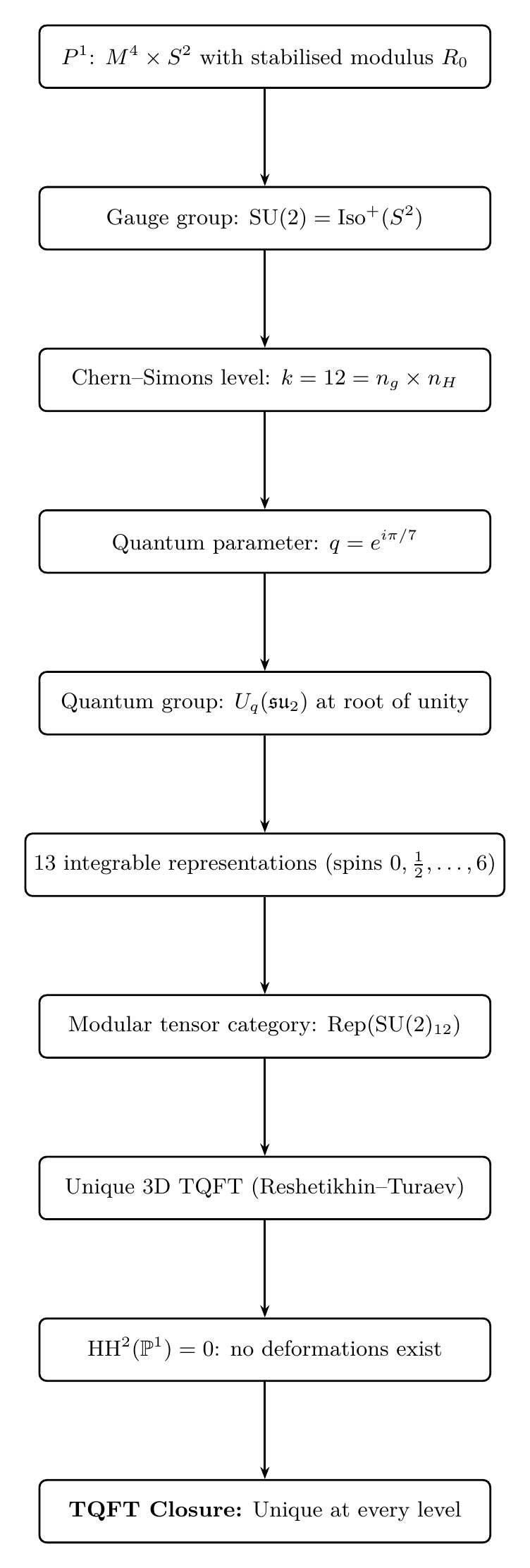
Chain summary:
Key results proven in this chapter:
- Atiyah–Segal axioms and TQFT functor structure (Theorem thm:168-tqft-axioms)
- 2D TQFT classification via Frobenius algebras; \(\dim Z(S^2) = 1\) (Theorem thm:168-dim-zs2)
- Chern–Simons at level \(k = 12\): five independent arguments (Theorem thm:168-k-equals-12)
- Central charge \(c = 18/7\) (Proposition prop:168-central-charge)
- Quantum group \(U_q(\mathfrak{su}_2)\): Hopf algebra structure (Theorem thm:168-uq-definition)
- Root of unity: 13 integrable representations (Theorem thm:168-root-of-unity)
- Quantum integers \([n]_q = \sin(n\pi/14)/\sin(\pi/14)\) (Theorem thm:168-quantum-integers)
- Modular tensor category \(\mathrm{Rep}(\mathrm{SU}(2)_{12})\) (Theorem thm:168-mtc)
- Reshetikhin–Turaev construction: unique 3D TQFT (Theorem thm:168-reshetikhin-turaev)
- Deformation rigidity: \(\mathrm{HH}^2(\mathbb{P}^1) = 0\) (Theorem thm:168-hh2-vanishing)
- \(q = e^{i\pi/7}\) is locked (Corollary cor:168-q-locked)
- Monopole–Wilson correspondence (Theorem thm:168-monopole-wilson)
- Jones polynomial at \(q = e^{i\pi/7}\): values in \(\mathbb{Q}(\zeta_{14})\) (Proposition prop:168-coloured-jones-k12)
- TMT factorization algebra (Theorem thm:168-tmt-factorization)
- Extended TQFT via cobordism hypothesis (Theorem thm:168-tmt-extended)
- Quasi-topological structure (Theorem thm:168-quasi-topological)
- TQFT Closure Theorem: uniqueness at every level (Theorem thm:168-tqft-closure)
Cross-references:
- \(P^1\) and \(S^2\) geometry \(\longrightarrow\) Chapter 3 (Geometric Foundation)
- Gauge group \(\mathrm{SU}(2)\) from \(\mathrm{Iso}(S^2)\) \(\longrightarrow\) Chapter 3
- Monopole harmonics \(Y_\ell m}\) \(\longrightarrow\) Chapter 7 (Monopole Harmonics)
- Deformation rigidity \(\mathrm{HH}^2(\mathbb{P}^1) = 0\) \(\longrightarrow\) Chapters 161, 171 (Algebraic Geometry)
- Modulus stabilisation fixing \(R_0\) \(\longrightarrow\) Chapter 117 (Modulus Stabilisation)
- Number-theoretic closure (primes \(\{2, 3, 5, 7\}) \(\longrightarrow\) Chapter 167 (Class Field Theory)
- Motivic structure \(h(\mathbb{CP}^1)\) \(\longrightarrow\) Chapter 165 (Motives)
Verification Code
The mathematical derivations and proofs in this chapter can be independently verified using the formal and computational scripts below.
All verification code is open source. See the complete verification index for all chapters.