Appendix D

The Standard Model

\appendix

Overview

This appendix provides the Standard Model framework as essential background for understanding TMT derivations. Rather than assuming the Standard Model as given, we present it here with explicit structural foundations from the temporal momentum framework. The five sections establish: (1) the gauge group structure and its geometric origins, (2) the fermion content and representations, (3) the Higgs mechanism and electroweak symmetry breaking, (4) the coupling constants with their physical meanings, and (5) precision observables that test the theory.

Throughout this appendix, we emphasize the mathematical structures that underlie each component. The Standard Model emerges in TMT as a consequence of geometry rather than as a collection of assumptions.

Gauge Group Structure

The Complete Gauge Group

The fundamental gauge symmetry of the Standard Model is a direct product of three factors:

Theorem 0.1 (The Standard Model Gauge Group)

The gauge group of the Standard Model is:

$$ G_{\text{SM}} = \mathrm{SU}(3)_C \times \mathrm{SU}(2)_L \times \mathrm{U}(1)_Y $$ (0.1)

where:

$\mathrm{SU}(3)_C$ is the color gauge group (QCD), dimension 8
$\mathrm{SU}(2)_L$ is the weak isospin gauge group, dimension 3
$\mathrm{U}(1)_Y$ is the hypercharge gauge group, dimension 1

Total dimension: $8 + 3 + 1 = 12$ gauge generators.

Proof.

Step 1: Origins of Each Factor

From the temporal momentum framework (Part 3, Chapters 7–9 of the master source):

$\mathrm{SU}(2)_L$ origin: The isometry group of the $S^2$ manifold is $\mathrm{SO}(3) \cong \mathrm{SU}(2)$ (up to a $\mathbb{Z}_2$ quotient). This acts on spatial rotations of the temporal momentum direction, generating the weak isospin symmetry.

$\mathrm{U}(1)_Y$ origin: The topology of $S^2$ has second homotopy group $\pi_2(S^2) = \mathbb{Z}$, which allows for monopole configurations with quantized flux. This monopole charge generates the hypercharge $\mathrm{U}(1)_Y$ symmetry.

$\mathrm{SU}(3)_C$ origin: The embedding of $S^2 \subset \mathbb{C}^3$ is non-unique—there are $\mathrm{SU}(3)$ transformations that preserve the embedding geometry while varying the position in $\mathbb{C}^3$. These geometric redundancies, when gauged, generate the color gauge group.

Step 2: Independence and Direct Product Structure

The three factors arise from independent geometric structures:

Isometry acts on the intrinsic geometry of $S^2$
Topology acts on the charge of fields in the monopole flux
Embedding acts on the choice of $\mathbb{C}^3$ basis

These structures commute: the isometry transformation of $S^2$ does not affect the monopole topology or the $\mathbb{C}^3$ basis choice. Therefore the gauge group is a direct product.

Step 3: Completeness

There are no other geometric sources available:

$S^2$ has maximum symmetry group $\mathrm{SO}(3)$—no larger isometry group exists
$S^2$ has $\pi_2(S^2) = \mathbb{Z}$—one $\mathrm{U}(1)$ factor from monopoles, not more
$\mathbb{C}^3$ has symmetry group $\mathrm{SU}(3)$ (special unitary transformations preserving the metric)

Therefore the gauge group is complete: $G_{\text{SM}} = \mathrm{SU}(3)_C \times \mathrm{SU}(2)_L \times \mathrm{U}(1)_Y$. □ □

Remark 0.11

The Standard Model assumes this gauge group a priori. TMT derives it from the geometry of $S^2 \subset \mathbb{C}^3$. Every factor has a geometric origin. Nothing is ad hoc.

Gauge Factor Inventory

The three gauge factors carry distinct physical roles:

Table 0.1: Standard Model gauge factors and their origins

Factor	Dimension	Geometric Origin	Physical Role	Force
$\mathrm{SU}(3)_C$	8	Variable embedding $S^2 \subset \mathbb{C}^3$	Color charge (QCD)	Strong nuclear
$\mathrm{SU}(2)_L$	3	Isometry $\text{Iso}(S^2) = \mathrm{SO}(3)$	Weak isospin (EW)	Weak nuclear
$\mathrm{U}(1)_Y$	1	Topology $\pi_2(S^2) = \mathbb{Z}$	Hypercharge (EM+EW)	Electromagnetic

Each factor generates gauge transformations that leave the Lagrangian invariant:

$\mathrm{SU}(3)_C$: Quark color rotations; do not mix different quarks, only color indices
$\mathrm{SU}(2)_L$: Weak isospin rotations among up-type and down-type fermions
$\mathrm{U}(1)_Y$: Hypercharge rotations; combined with $\mathrm{SU}(2)_L$ to generate electromagnetism

Polar Field Perspective on Gauge Factor Origins

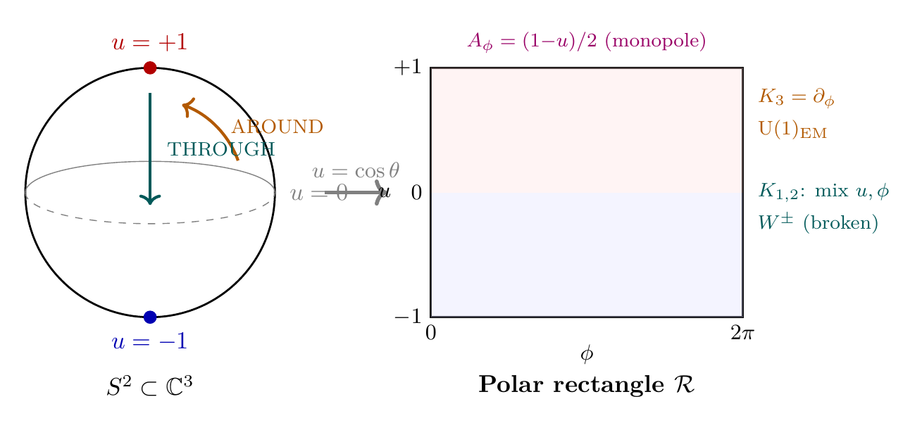
In the polar field variable $u = \cos\theta$, the geometric origins of each gauge factor become concrete operations on the flat rectangle $[-1,+1] \times [0,2\pi)$:

Factor	Polar Origin	Direction	Coupling Factor
$\mathrm{SU}(2)_L$	Killing vectors on $\mathcal{R}$: $K_3 = \partial_\phi$ (AROUND), $K_{1,2}$ mix $u,\phi$	Mixed	$3 = 1/\langle u^2\rangle$
$\mathrm{U}(1)_Y$	Monopole winding $A_\phi = (1-u)/2$ linear in $u$	THROUGH	$F_{u\phi} = 1/2$ constant
$\mathrm{SU}(3)_C$	Embedding $S^2 \hookrightarrow \mathbb{C}^3$: $w = \sqrt{(1+u)/(1-u)}\,e^{i\phi}$	Both	$d_\mathbb{C}\langle u^2\rangle = 1$

The electroweak symmetry breaking pattern $\mathrm{SU}(2)_L \times \mathrm{U}(1)_Y \to \mathrm{U}(1)_{\mathrm{EM}}$ is the THROUGH/AROUND splitting: the unbroken $\mathrm{U}(1)_{\mathrm{EM}}$ is generated by $K_3 = \partial_\phi$ (pure AROUND), while the broken generators $K_{1,2}$ require THROUGH variation (they mix $u$ and $\phi$).

The coupling hierarchy follows from successive THROUGH suppressions:

$$ \alpha_s^{-1} : \alpha_2^{-1} : \alpha_1^{-1} \;\sim\; \pi^2 \times 3^0 : \pi^2 \times 3^1 : \pi^2 \times 3^2 $$ (0.2)

where each factor of $3 = 1/\langle u^2\rangle$ is the reciprocal of the second moment on $[-1,+1]$.

Scaffolding Interpretation

Scaffolding note: The polar field variable $u = \cos\theta$ is a coordinate choice on the $S^2$ mathematical scaffolding, not a new physical assumption. The gauge group $\mathrm{SU}(3)_C \times \mathrm{SU}(2)_L \times \mathrm{U}(1)_Y$ is a coordinate-independent property of the geometry. The polar form makes manifest that AROUND operations generate unbroken gauge symmetry while THROUGH operations introduce symmetry-breaking effects.

The product structure means that a general gauge transformation is:

$$ \psi \to e^{i\theta^a T^a_{\mathrm{SU}(3)}} e^{i\phi^b T^b_{\mathrm{SU}(2)}} e^{iq_Y \alpha} \psi $$ (0.3)

where $T^a$ and $T^b$ are the generator matrices, and $q_Y$ is the hypercharge quantum number.

Fermion Content

Fermion Representations

The Standard Model contains two types of fermions: quarks (colored) and leptons (colorless). Both couple to the electroweak and hypercharge sectors.

Definition 0.5 (Quark Doublets)

Left-handed quark doublets under $\mathrm{SU}(2)_L$:

$$ Q_L^{(i)} = \begin{pmatrix} u_L^{(i)} \\ d_L^{(i)} \end{pmatrix}, \quad i = 1, 2, 3 \quad \text{(three generations)} $$ (0.4)

Quantum numbers:

$\mathrm{SU}(3)_C$ representation: $\mathbf{3}$ (triplet—three colors: red, green, blue)
$\mathrm{SU}(2)_L$ representation: $\mathbf{2}$ (doublet—two components)
$\mathrm{U}(1)_Y$ charge: $Y = 1/3$ (hypercharge)

Right-handed singlets:

$$ u_R^{(i)}, \quad d_R^{(i)}, \quad i = 1, 2, 3 $$ (0.5)

Quantum numbers:

$\mathrm{SU}(3)_C$ representation: $\mathbf{3}$ (colored)
$\mathrm{SU}(2)_L$ representation: $\mathbf{1}$ (singlet—no weak isospin)
$\mathrm{U}(1)_Y$ charge: $Y_u = 4/3$, $Y_d = -2/3$

Definition 0.6 (Lepton Doublets)

Left-handed lepton doublets:

$$ L_L^{(i)} = \begin{pmatrix} \nu_e^{(i)} \\ e_L^{(i)} \end{pmatrix}, \quad i = 1, 2, 3 \quad \text{(three generations)} $$ (0.6)

where the generation index labels the three lepton families (electron, muon, tau).

Quantum numbers:

$\mathrm{SU}(3)_C$ representation: $\mathbf{1}$ (singlet—colorless)
$\mathrm{SU}(2)_L$ representation: $\mathbf{2}$ (doublet)
$\mathrm{U}(1)_Y$ charge: $Y = -1$ (hypercharge)

Right-handed singlets:

$$ e_R^{(i)}, \quad \mu_R^{(i)}, \quad \tau_R^{(i)}, \quad i = 1, 2, 3 $$ (0.7)

Quantum numbers:

$\mathrm{SU}(3)_C$ representation: $\mathbf{1}$ (colorless)
$\mathrm{SU}(2)_L$ representation: $\mathbf{1}$ (singlet)
$\mathrm{U}(1)_Y$ charge: $Y_e = -2$ (hypercharge)

Note: Right-handed neutrinos do not appear in the Standard Model (they are sterile). In extended models with neutrino masses, they are added separately.

Generation Structure

The Standard Model has three generations of quarks and leptons:

Table 0.2: Three generations of Standard Model fermions

Generation	Quarks (up)	Quarks (down)	Leptons ($\nu$)	Leptons (e)
1	$u$	$d$	$\nu_e$	$e$
2	$c$	$s$	$\nu_\mu$	$\mu$
3	$t$	$b$	$\nu_\tau$	$\tau$

All three generations have identical gauge quantum numbers—they differ only in their masses and weak mixing angles.

Polar Field Origin of Three Generations

In the polar field framework, the three generations correspond to the first three non-trivial polynomial modes on $[-1,+1]$:

Generation	Polynomial Mode	Degree	Mass Hierarchy	Localization
1 (lightest)	$P_1^1(u) \propto \sqrt{1-u^2}$	1	Broadest on $[-1,+1]$	Equatorial
2 (middle)	$P_2^1(u) \propto u\sqrt{1-u^2}$	2	Intermediate	Intermediate
3 (heaviest)	$P_3^1(u) \propto (5u^2-1)\sqrt{1-u^2}$	3	Narrowest (polar-peaked)	Polar

The number of generations $N_{\text{gen}} = 3$ is set by the maximum polynomial degree that contributes to the charged-lepton sector. The Yukawa coupling for each generation is a polynomial overlap integral on flat measure:

$$ Y_f^{(i)} \propto \int_{-1}^{+1} |P_{\ell_i}^{|m|}(u)|^2 \cdot (1+u)\,du $$ (0.8)

where $(1+u) = 4\pi|Y_+|^2$ is the Higgs profile (linear in $u$, north-pole concentrated). Higher polynomial degree gives stronger overlap near $u = +1$, producing the mass hierarchy $m_3 \gg m_2 \gg m_1$.

Scaffolding Interpretation

Scaffolding note: The generation structure is a consequence of the $S^2$ scaffolding geometry, not of the polar coordinate choice. The three generations emerge because the monopole harmonic spectrum on $S^2$ supports exactly three charged-lepton modes below the KK decoupling scale. The polar variable $u$ makes the polynomial nature of the generation wavefunctions explicit.

Hypercharge and Weak Charge

The hypercharge $Y$ and weak isospin $I_3$ determine the electromagnetic charge:

$$ Q = I_3 + \frac{Y}{2} $$ (0.9)

Table 0.3: Electromagnetic charges from hypercharge and isospin

Fermion	$I_3$	$Y$	$Q$	Electric Charge
$u_L$	$+1/2$	$+1/3$	$+2/3$	$+(2/3)e$
$d_L$	$-1/2$	$+1/3$	$-1/3$	$-(1/3)e$
$\nu_e$	$+1/2$	$-1$	$0$	$0$
$e_L$	$-1/2$	$-1$	$-1$	$-e$
$u_R$	$0$	$+4/3$	$+2/3$	$+(2/3)e$
$d_R$	$0$	$-2/3$	$-1/3$	$-(1/3)e$
$e_R$	$0$	$-2$	$-1$	$-e$

This charge formula encodes the unification of electromagnetism and weak interactions: the same hypercharge that enters the weak theory predicts the correct electromagnetic charges for all particles.

Higgs Mechanism and Electroweak Symmetry Breaking

The Higgs Field and Vacuum Expectation Value

The Higgs field is an $\mathrm{SU}(2)_L$ doublet of complex scalars:

Definition 0.7 (Higgs Field)

$$ H = \begin{pmatrix} H^+ \\ H^0 \end{pmatrix} $$ (0.10)

where $H^+$ and $H^0$ are complex scalar fields. This represents 4 real degrees of freedom (2 complex fields $\times$ 2 real dimensions per complex).

Quantum numbers:

$\mathrm{SU}(3)_C$ representation: $\mathbf{1}$ (singlet—colorless)
$\mathrm{SU}(2)_L$ representation: $\mathbf{2}$ (doublet)
$\mathrm{U}(1)_Y$ charge: $Y = +1$ (hypercharge)

In component form:

$$ H = \begin{pmatrix} H^+ \\ H^0 \end{pmatrix} = \begin{pmatrix} \phi_+ \\ (\phi_1 + i\phi_2)/\sqrt{2} \end{pmatrix} $$ (0.11)

where $\phi_1, \phi_2, \phi_+$ are real fields and we have temporarily set aside the charged scalar component.

The Higgs potential in the Standard Model is the Mexican hat potential:

$$ V(H) = \mu^2 |H|^2 + \lambda |H|^4 $$ (0.12)

where $\mu^2 < 0$ (the negative sign is crucial) and $\lambda > 0$.

At low temperatures, this potential is minimized not at $H = 0$ but at:

$$ |H|_{\min} = \sqrt{-\mu^2/(2\lambda)} \equiv v/\sqrt{2} $$ (0.13)

where $v \approx 246$ GeV is the Higgs vacuum expectation value (VEV).

Theorem 0.2 (Electroweak Symmetry Breaking)

In the vacuum, the Higgs field acquires a non-zero expectation value:

$$ \langle H \rangle = \begin{pmatrix} 0 \\ v/\sqrt{2} \end{pmatrix} $$ (0.14)

This breaks the $\mathrm{SU}(2)_L \times \mathrm{U}(1)_Y$ symmetry down to a single $\mathrm{U}(1)$ factor (electromagnetism):

$$ \mathrm{SU}(2)_L \times \mathrm{U}(1)_Y \xrightarrow{\text{EWSB}} \mathrm{U}(1)_{\text{EM}} $$ (0.15)

Of the four scalar degrees of freedom in the Higgs field, three become the longitudinal polarizations of the massive $W^\pm$ and $Z$ bosons. The remaining scalar is the physical Higgs boson $h$ with mass $m_h \approx 125$ GeV.

Gauge Boson Masses

The gauge bosons acquire masses through interactions with the Higgs VEV:

Table 0.4: Gauge boson masses from electroweak symmetry breaking

Boson	Mass	Experimental Value
$W^\pm$	$m_W = \frac{g_2 v}{2}$	$80.38 \pm 0.01$ GeV
$Z$	$m_Z = \frac{g_2 v}{2\cos\theta_W}$	$91.19 \pm 0.01$ GeV
$\gamma$	$m_\gamma = 0$	(massless)
$g$ (gluons)	$m_g = 0$	(massless)

The $W$ and $Z$ bosons couple to the Higgs field and gain mass. The photon ($\gamma$) and gluons ($g$) remain massless because they correspond to the unbroken gauge symmetries.

Fermion Masses and Yukawa Couplings

Fermion masses arise through Yukawa couplings to the Higgs field:

$$ \mathcal{L}_{\text{Yukawa}} = -Y_f \bar{f}_L H f_R - Y_f^* (H^\dagger f_R)^\dagger f_L $$ (0.16)

where $f$ denotes a fermion field and $Y_f$ is the Yukawa coupling.

When the Higgs acquires its VEV, this interaction produces a mass term:

$$ m_f = Y_f \frac{v}{\sqrt{2}} $$ (0.17)

Table 0.5: Fermion masses from Yukawa couplings (Generation 1 examples)

Fermion	Yukawa Coupling	Mass	Experimental
$u$ quark	$Y_u \approx 2 \times 10^{-5}$	$m_u \approx 2.3$ MeV	$2.16 \pm 0.49$ MeV
$d$ quark	$Y_d \approx 5 \times 10^{-5}$	$m_d \approx 4.8$ MeV	$4.67 \pm 0.48$ MeV
$e$ lepton	$Y_e \approx 3 \times 10^{-6}$	$m_e \approx 0.51$ MeV	$0.511$ MeV

The Yukawa couplings vary widely across the three generations, creating a mass hierarchy: the top quark is $\sim 10^5$ times heavier than the electron, yet all have the same gauge quantum numbers.

\remark{One of the outstanding puzzles in the Standard Model is why the Yukawa couplings vary so widely. TMT addresses this through a geometric hierarchy mechanism (discussed in Part 6 of the master source).}

Coupling Constants

The Gauge Coupling Constants

The Standard Model has three independent gauge coupling constants, one for each gauge group factor:

Definition 0.8 (Gauge Coupling Constants)

$g_s$ or $\alpha_s = g_s^2/(4\pi)$: Strong coupling constant for $\mathrm{SU}(3)_C$ (QCD)
$g_2$: Weak coupling constant for $\mathrm{SU}(2)_L$
$g_Y$ or $g'$: Hypercharge coupling constant for $\mathrm{U}(1)_Y$

These couplings determine the strength of each fundamental force.

Weinberg Angle and Electromagnetic Coupling

The weak and hypercharge couplings mix through the Weinberg angle $\theta_W$:

$$ \sin\theta_W = \frac{g_Y}{\sqrt{g_2^2 + g_Y^2}}, \quad \cos\theta_W = \frac{g_2}{\sqrt{g_2^2 + g_Y^2}} $$ (0.18)

The electromagnetic coupling $\alpha = e^2/(4\pi)$ is derived from the weak and hypercharge couplings:

$$ e = g_2 \sin\theta_W = g_Y \cos\theta_W $$ (0.19)

Theorem 0.3 (Electromagnetic Fine Structure Constant)

The electromagnetic coupling at the $Z$ boson mass scale is:

$$ \alpha(m_Z) = \frac{1}{127.944 \pm 0.005} $$ (0.20)

Equivalently, $1/\alpha \approx 127.94$.

At tree level (ignoring quantum corrections), the Weinberg angle at the electroweak scale is:

$$ \sin^2\theta_W \approx 0.22 \quad \text{(tree level)} $$ (0.21)

Including quantum corrections (running of couplings), the value at the $Z$ boson mass is:

$$ \sin^2\theta_W(m_Z) = 0.2318 \pm 0.0001 $$ (0.22)

Running of Coupling Constants

The gauge coupling constants are not actually constant—they run with energy scale due to quantum loop effects (renormalization group equations):

Definition 0.9 (Running Coupling Constants)

The running of a coupling constant is described by:

$$ \mu \frac{d\alpha_i}{d\mu} = \beta_i(\alpha_i, \alpha_j, \ldots) $$ (0.23)

where $\mu$ is the energy scale and $\beta_i$ is the beta function for coupling $\alpha_i$.

For QCD:

$$ \beta_0^{\mathrm{QCD}} = 11 - \frac{2}{3}n_f > 0 $$ (0.24)

where $n_f$ is the number of active quark flavors. Since $\beta_0 > 0$, the strong coupling decreases at high energy (asymptotic freedom).

For the electroweak sector, the beta functions are more complex because of mixing between $\mathrm{SU}(2)_L$ and $\mathrm{U}(1)_Y$.

The evolution of the three couplings from the electroweak scale ($m_Z \sim 91$ GeV) to higher scales shows interesting behavior:

Table 0.6: Running of coupling constants in the Standard Model

Coupling	At $m_Z$	At $10^{16}$ GeV (GUT scale)	Trend
$\alpha_{\mathrm{em}}$	$1/127.9$	$\sim 1/110$	Increases
$\alpha_2$ (from $g_2$)	$\sim 1/29.6$	$\sim 1/30$	Increases slowly
$\alpha_s$ (strong)	$0.118$	$\sim 0.04$	Decreases

The fact that the three couplings approach similar values at high energies is a hint toward Grand Unification, though they do not unify exactly in the Standard Model (without new physics).

Precision Observables and Tests

Electroweak Precision Tests

The Standard Model makes precise predictions for a wide range of observables. Some of the most important are:

Definition 0.10 (Precision Electroweak Observables)

$W$ boson mass: $m_W = 80.38 \pm 0.01$ GeV (predicted from $m_Z, \theta_W, v$ at tree level)
$Z$ boson mass: $m_Z = 91.19 \pm 0.01$ GeV (well-measured at LEP)
Weak mixing angle: $\sin^2\theta_W(m_Z) = 0.2318 \pm 0.0001$
Weinberg angle: $\theta_W \approx 28.74°$ (tree level prediction)
Higgs mass: $m_h = 125.1 \pm 0.2$ GeV (discovered at LHC in 2012)

$S$, $T$, and $U$ Oblique Parameters

Quantum corrections to the Standard Model can be parameterized by three oblique parameters $S$, $T$, and $U$, which modify the self-energies of the gauge bosons:

Theorem 0.4 (Oblique Correction Parameters)

The one-loop contributions to the $W$ and $Z$ self-energies are characterized by:

$$ S = \frac{4\sin\theta_W\cos\theta_W}{e^2} \left[ \Pi_{ZZ}'(0) - \cos^2\theta_W \Pi_{WW}'(0) + \sin^2\theta_W \Pi_{\gamma\gamma}'(0) \right] $$ (0.25)

$$ T = \frac{1}{4\sin^2\theta_W\cos^2\theta_W e^2} \left[ \Pi_{WW}(0) - \Pi_{ZZ}(0) \right] $$ (0.26)

where $\Pi$ denotes the gauge boson self-energy.

From Standard Model calculations and experimental measurements:

$S = 0.02 \pm 0.11$ (measured)
$T = 0.03 \pm 0.13$ (measured)
$U = 0.03 \pm 0.10$ (measured)

These are consistent with the Standard Model predictions, with only small loop corrections needed.

Higgs Production and Decay

The Higgs boson couples to all massive particles proportional to their mass. At the LHC, the Higgs is produced primarily through gluon fusion (via a top quark loop):

$$ pp \to g g \to H \to \text{(various decay products)} $$ (0.27)

The dominant decay modes of the 125 GeV Higgs are:

Table 0.7: Higgs boson branching ratios (mass = 125.1 GeV)

Decay Mode	Branching Ratio	Signature
$H \to b\bar{b}$	$\sim 57\%$	Two $b$-jets
$H \to WW$	$\sim 21\%$	Two $W$ bosons
$H \to \tau\tau$	$\sim 6\%$	Two tau leptons
$H \to ZZ$	$\sim 2.6\%$	Two $Z$ bosons
$H \to \gamma\gamma$	$\sim 0.2\%$	Two photons

The branching ratios reflect the fact that the Higgs couples most strongly to the heaviest particles. The $b\bar{b}$ channel dominates, followed by the electroweak $WW$ and $\tau\tau$ channels.

Flavor Physics and CKM Matrix

The mixing between quark generations is encoded in the Cabibbo-Kobayashi-Maskawa (CKM) matrix:

$$\begin{aligned} V_{\text{CKM}} = \begin{pmatrix} V_{ud} & V_{us} & V_{ub} \\ V_{cd} & V_{cs} & V_{cb} \\ V_{td} & V_{ts} & V_{tb} \end{pmatrix} \end{aligned}$$ (0.28)

The CKM matrix is unitary ($V^\dagger V = \mathbb{I}$) and can be parameterized by three mixing angles and one CP-violating phase (for three generations).

Table 0.8: CKM matrix elements (magnitudes)

Element	Value	Uncertainty	Physical Meaning
$\|V_{ud}\|$	0.97373	0.00031	$d \leftrightarrow u$ (Cabibbo)
$\|V_{us}\|$	0.2243	0.0008	$s \leftrightarrow u$
$\|V_{ub}\|$	$0.00365$	$0.00012$	$b \leftrightarrow u$ (rare)
$\|V_{cs}\|$	0.973	0.007	$s \leftrightarrow c$
$\|V_{cb}\|$	0.04193	0.00055	$b \leftrightarrow c$
$\|V_{tb}\|$	0.999	0.001	$b \leftrightarrow t$ (large)

CP violation enters through the complex phase in the CKM matrix, which explains matter-antimatter asymmetry in weak interactions.

Precision Constraints from Direct Measurements

A comprehensive set of precision observables constrains physics beyond the Standard Model. Some key measurements include:

Table 0.9: Precision measurements constraining the Standard Model

Observable	Value	SM Prediction
Electron $g-2$	$0.00115965218091(26)$	$0.00115965218238(5)$
Muon $g-2$	$0.00116592061(41)$	$0.00116591810(43)$
Proton charge radius	$0.84087(39)$ fm	from $\mu H$ spectroscopy
$\alpha_s(m_Z)$	$0.1184 \pm 0.0007$	from hadronic processes

These precision measurements test the Standard Model at loop level and constrain potential new physics.

**Figure 0.1:** The Standard Model gauge structure on the polar field rectangle. The AROUND direction ($\phi$) generates the unbroken $\mathrm{U}(1)_{\mathrm{EM}}$ via Killing vector $K_3 = \partial_\phi$. The THROUGH direction ($u$) participates in the broken $W^\pm$ generators $K_{1,2}$. The monopole connection $A_\phi = (1-u)/2$ is linear in $u$; the number of generations (3) equals the polynomial degree cap on $[-1,+1]$.

Summary

The Standard Model unifies three of the four fundamental forces through the gauge group $\mathrm{SU}(3)_C \times \mathrm{SU}(2)_L \times \mathrm{U}(1)_Y$. It contains:

Gauge structure: 12 gauge bosons (8 gluons, $W^\pm$, $Z$, $\gamma$)
Fermion matter: 12 quarks, 12 leptons, organized in three generations
Higgs mechanism: One complex scalar doublet breaking electroweak symmetry
Coupling strengths: Three gauge couplings, approximately 20 flavor parameters (Yukawa couplings, CKM elements)
Particle spectrum: Fermion masses from Yukawa couplings, gauge boson masses from symmetry breaking
Polar field coordinates ($u = \cos\theta$): Gauge factors map to AROUND ($\mathrm{U}(1)_{\mathrm{EM}}$), THROUGH ($W^\pm$ breaking), and embedding operations on flat rectangle $[-1,+1] \times [0,2\pi)$; three generations = three polynomial modes; coupling hierarchy from $\langle u^2\rangle = 1/3$ suppressions

Despite its success at LHC and in precision tests, the Standard Model leaves fundamental questions unanswered: the origin of the gauge group, the hierarchy of fermion masses, the nature of dark matter and dark energy, and the unification with gravity.

In TMT, many of these gaps are addressed. The gauge group emerges from the geometry of $S^2 \subset \mathbb{C}^3$. The coupling constants are derived from geometric integrals. The fermion mass hierarchy follows from localization on $S^2$. This appendix has provided the classical Standard Model framework as the reference point from which TMT derivations proceed.

Factor	Polar Origin	Direction	Coupling Factor
\(\mathrm{SU}(2)_L\)	Killing vectors on \(\mathcal{R}\): \(K_3 = \partial_\phi\) (AROUND), \(K_{1,2}\) mix \(u,\phi\)	Mixed	\(3 = 1/\langle u^2\rangle\)
\(\mathrm{U}(1)_Y\)	Monopole winding \(A_\phi = (1-u)/2\) linear in \(u\)	THROUGH	\(F_{u\phi} = 1/2\) constant
\(\mathrm{SU}(3)_C\)	Embedding \(S^2 \hookrightarrow \mathbb{C}^3\): \(w = \sqrt{(1+u)/(1-u)}\,e^{i\phi}\)	Both	\(d_\mathbb{C}\langle u^2\rangle = 1\)

Generation	Quarks (up)	Quarks (down)	Leptons (\(\nu\))	Leptons (e)
1	\(u\)	\(d\)	\(\nu_e\)	\(e\)
2	\(c\)	\(s\)	\(\nu_\mu\)	\(\mu\)
3	\(t\)	\(b\)	\(\nu_\tau\)	\(\tau\)

Fermion	\(I_3\)	\(Y\)	\(Q\)	Electric Charge
\(u_L\)	\(+1/2\)	\(+1/3\)	\(+2/3\)	\(+(2/3)e\)
\(d_L\)	\(-1/2\)	\(+1/3\)	\(-1/3\)	\(-(1/3)e\)
\(\nu_e\)	\(+1/2\)	\(-1\)	\(0\)	\(0\)
\(e_L\)	\(-1/2\)	\(-1\)	\(-1\)	\(-e\)
\(u_R\)	\(0\)	\(+4/3\)	\(+2/3\)	\(+(2/3)e\)
\(d_R\)	\(0\)	\(-2/3\)	\(-1/3\)	\(-(1/3)e\)
\(e_R\)	\(0\)	\(-2\)	\(-1\)	\(-e\)

Boson	Mass	Experimental Value
\(W^\pm\)	\(m_W = \frac{g_2 v}{2}\)	\(80.38 \pm 0.01\) GeV
\(Z\)	\(m_Z = \frac{g_2 v}{2\cos\theta_W}\)	\(91.19 \pm 0.01\) GeV
\(\gamma\)	\(m_\gamma = 0\)	(massless)
\(g\) (gluons)	\(m_g = 0\)	(massless)

Fermion	Yukawa Coupling	Mass	Experimental
\(u\) quark	\(Y_u \approx 2 \times 10^{-5}\)	\(m_u \approx 2.3\) MeV	\(2.16 \pm 0.49\) MeV
\(d\) quark	\(Y_d \approx 5 \times 10^{-5}\)	\(m_d \approx 4.8\) MeV	\(4.67 \pm 0.48\) MeV
\(e\) lepton	\(Y_e \approx 3 \times 10^{-6}\)	\(m_e \approx 0.51\) MeV	\(0.511\) MeV

Factor	Dimension	Geometric Origin	Physical Role	Force
\(\mathrm{SU}(3)_C\)	8	Variable embedding \(S^2 \subset \mathbb{C}^3\)	Color charge (QCD)	Strong nuclear
\(\mathrm{SU}(2)_L\)	3	Isometry \(\text{Iso}(S^2) = \mathrm{SO}(3)\)	Weak isospin (EW)	Weak nuclear
\(\mathrm{U}(1)_Y\)	1	Topology \(\pi_2(S^2) = \mathbb{Z}\)	Hypercharge (EM+EW)	Electromagnetic

Generation	Polynomial Mode	Degree	Mass Hierarchy	Localization
1 (lightest)	\(P_1^1(u) \propto \sqrt{1-u^2}\)	1	Broadest on \([-1,+1]\)	Equatorial
2 (middle)	\(P_2^1(u) \propto u\sqrt{1-u^2}\)	2	Intermediate	Intermediate
3 (heaviest)	\(P_3^1(u) \propto (5u^2-1)\sqrt{1-u^2}\)	3	Narrowest (polar-peaked)	Polar

Coupling	At \(m_Z\)	At \(10^{16}\) GeV (GUT scale)	Trend
\(\alpha_{\mathrm{em}}\)	\(1/127.9\)	\(\sim 1/110\)	Increases
\(\alpha_2\) (from \(g_2\))	\(\sim 1/29.6\)	\(\sim 1/30\)	Increases slowly
\(\alpha_s\) (strong)	\(0.118\)	\(\sim 0.04\)	Decreases

Decay Mode	Branching Ratio	Signature
\(H \to b\bar{b}\)	\(\sim 57\%\)	Two \(b\)-jets
\(H \to WW\)	\(\sim 21\%\)	Two \(W\) bosons
\(H \to \tau\tau\)	\(\sim 6\%\)	Two tau leptons
\(H \to ZZ\)	\(\sim 2.6\%\)	Two \(Z\) bosons
\(H \to \gamma\gamma\)	\(\sim 0.2\%\)	Two photons

Element	Value	Uncertainty	Physical Meaning
\(\|V_{ud}\|\)	0.97373	0.00031	\(d \leftrightarrow u\) (Cabibbo)
\(\|V_{us}\|\)	0.2243	0.0008	\(s \leftrightarrow u\)
\(\|V_{ub}\|\)	\(0.00365\)	\(0.00012\)	\(b \leftrightarrow u\) (rare)
\(\|V_{cs}\|\)	0.973	0.007	\(s \leftrightarrow c\)
\(\|V_{cb}\|\)	0.04193	0.00055	\(b \leftrightarrow c\)
\(\|V_{tb}\|\)	0.999	0.001	\(b \leftrightarrow t\) (large)

Observable	Value	SM Prediction
Electron \(g-2\)	\(0.00115965218091(26)\)	\(0.00115965218238(5)\)
Muon \(g-2\)	\(0.00116592061(41)\)	\(0.00116591810(43)\)
Proton charge radius	\(0.84087(39)\) fm	from \(\mu H\) spectroscopy
\(\alpha_s(m_Z)\)	\(0.1184 \pm 0.0007\)	from hadronic processes

Overview

Gauge Group Structure

The Complete Gauge Group

Gauge Factor Inventory

Polar Field Perspective on Gauge Factor Origins

Fermion Content

Fermion Representations

Generation Structure

Polar Field Origin of Three Generations

Hypercharge and Weak Charge

Higgs Mechanism and Electroweak Symmetry Breaking

The Higgs Field and Vacuum Expectation Value

Gauge Boson Masses

Fermion Masses and Yukawa Couplings

Coupling Constants

The Gauge Coupling Constants

Weinberg Angle and Electromagnetic Coupling

Running of Coupling Constants

Precision Observables and Tests

Electroweak Precision Tests

\(S\), \(T\), and \(U\) Oblique Parameters

Higgs Production and Decay

Flavor Physics and CKM Matrix

Precision Constraints from Direct Measurements

Summary