Chapter 81

Weak Measurements and Quantum Trajectories

Key Result

This chapter extends TMT's measurement theory beyond projective measurements to include weak measurements and continuous monitoring. In the S² framework, weak measurements correspond to partial projection—extracting information while minimally disturbing the system. The chapter establishes how anomalous weak values, quantum trajectories, and state smoothing all emerge naturally from the S² geometric structure.

Key Results:

Weak values arise from partial S² projection with post-selection
Anomalous weak values reflect geometric phase amplification, not paradox
Quantum trajectories are stochastic paths on S² driven by measurement back-action
State smoothing improves our knowledge of past S² configurations without retrocausality

Weak Measurement Theory

Standard quantum measurements are strong—they project the system onto an eigenstate, extracting maximum information but maximally disturbing the state. Weak measurements, introduced by Aharonov, Albert, and Vaidman (1988), extract partial information with minimal disturbance. This section develops weak measurement theory from first principles and establishes the TMT interpretation via S² geometry.

AAV Weak Value Formula

Definition 81.14 (Measurement Strength)

Consider a system $S$ coupled to a pointer $P$ via interaction Hamiltonian:

$$ H_{\text{int}} = g \, A_S \otimes P_P \, \delta(t - t_0) $$ (81.1)

where $A_S$ is the measured observable, $P_P$ is the pointer momentum, and $g$ is the coupling strength.

The measurement is:

Strong if $g \gg \Delta P / \Delta A$, where $\Delta P$ is the pointer momentum uncertainty and $\Delta A$ is the system observable spread
Weak if $g \ll \Delta P / \Delta A$

Observation 81.20 (Physical Interpretation of Strong vs Weak)

Strong measurement:

Pointer shifts by distinct amounts for each eigenvalue
System collapses to eigenstate
Full information extracted, maximum disturbance

Weak measurement:

Pointer shift much smaller than pointer uncertainty
System state barely disturbed
Partial information extracted, minimal disturbance
Individual results meaningless; statistics reveal “weak value”

Theorem 81.1 (Weak Value Formula)

For a system pre-selected in state $|\psi_i\rangle$ and post-selected in state $|\psi_f\rangle$, the weak value of observable $A$ is:

$$ \boxed{\langle A \rangle_w = \frac{\langle \psi_f | A | \psi_i \rangle}{\langle \psi_f | \psi_i \rangle}} $$ (81.2)

This is generally complex-valued. The real part determines the pointer position shift; the imaginary part determines the pointer momentum shift.

Theorem 81.2 (Pointer Shift from Weak Value)

For a weak measurement with Gaussian pointer state of width $\sigma$, the post-selected pointer position distribution is shifted by:

$$ \langle Q \rangle_{\text{post}} = g \cdot \text{Re}\langle A \rangle_w $$ (81.3)

and the pointer momentum distribution is shifted by:

$$ \langle P \rangle_{\text{post}} = \frac{g}{\sigma^2} \cdot \text{Im}\langle A \rangle_w $$ (81.4)

Proof.

Step 1: Initial State The combined system-pointer state is:

$$ |\Psi_i\rangle = |\psi_i\rangle \otimes |\phi_P\rangle $$ (81.5)

where the pointer state is a Gaussian: $\phi_P(q) = (\pi\sigma^2)^{-1/4} e^{-q^2/2\sigma^2}$.

Step 2: After Interaction The unitary evolution gives:

$$ |\Psi\rangle = e^{-igAP/\hbar}|\psi_i\rangle \otimes |\phi_P\rangle $$ (81.6)

Step 3: Weak Coupling Expansion For weak coupling ($g \ll 1$), expand to first order in $g$:

$$ |\Psi\rangle \approx \left(1 - \frac{ig}{\hbar}AP\right)|\psi_i\rangle \otimes |\phi_P\rangle $$ (81.7)

Step 4: Post-Selection Projecting onto $|\psi_f\rangle$ gives:

$$\begin{aligned} \langle\psi_f|\Psi\rangle &\approx \langle\psi_f|\psi_i\rangle \left(1 - \frac{ig}{\hbar}\frac{\langle\psi_f|A|\psi_i\rangle}{\langle\psi_f|\psi_i\rangle}P\right)|\phi_P\rangle \\ &= \langle\psi_f|\psi_i\rangle \left(1 - \frac{ig}{\hbar}\langle A\rangle_w P\right)|\phi_P\rangle \end{aligned}$$ (81.41)

Step 5: Pointer Shift The operator $(1 - ig\langle A\rangle_w P/\hbar)$ acts on the Gaussian pointer by shifting its center:

Position shift: $\Delta Q = g \cdot \text{Re}\langle A\rangle_w$
Momentum shift: $\Delta P = (g/\sigma^2) \cdot \text{Im}\langle A\rangle_w$

Both shifts are proportional to the weak value, with the sign of the coupling $g$ determining the shift direction. $\blacksquare$ □

Pre- and Post-Selection

Definition 81.15 (Filtered and Smoothed States)

In weak measurement protocols:

Pre-selection: The system is prepared in state $|\psi_i\rangle$ at $t=0$.

Weak measurement: Observable $A$ is weakly coupled at time $t_0$.

Post-selection: The system is measured to be in state $|\psi_f\rangle$ at time $t_f > t_0$.

The weak value $\langle A \rangle_w$ is extracted only from those experimental runs where post-selection succeeds. This creates a biased sub-ensemble.

Theorem 81.3 (TMT Interpretation: Partial S² Projection)

In TMT, the weak value arises from partial projection on S²:

Let $|\psi_i\rangle$ correspond to wave function $\psi_i(\Omega)$ on S², and let post-selection $|\psi_f\rangle$ select the region $\Omega_f \subset S^2{}$. Then:

$$ \boxed{\langle A \rangle_w = \frac{\int_{S^2{}} \psi_f^*(\Omega) \, A(\Omega) \, \psi_i(\Omega) \, d\Omega}{\int_{S^2{}} \psi_f^*(\Omega) \, \psi_i(\Omega) \, d\Omega}} $$ (81.8)

For localized post-selection around $\Omega_f$:

$$ \langle A \rangle_w \approx \frac{\int_{\Omega_f} A(\Omega) \, \psi_i(\Omega) \, d\Omega}{\int_{\Omega_f} \psi_i(\Omega) \, d\Omega} $$ (81.9)

Proof.

The standard weak value formula $\langle A \rangle_w = \langle\psi_f|A|\psi_i\rangle / \langle\psi_f|\psi_i\rangle$ becomes, in the S² representation:

Numerator:

$$ \langle\psi_f|A|\psi_i\rangle = \int_{S^2{}} \psi_f^*(\Omega) \, A(\Omega) \, \psi_i(\Omega) \, d\Omega $$ (81.10)

Denominator:

$$ \langle\psi_f|\psi_i\rangle = \int_{S^2{}} \psi_f^*(\Omega) \, \psi_i(\Omega) \, d\Omega $$ (81.11)

The ratio gives Eq. eq:60n-weak-value-s2. The localized approximation (Eq. eq:60n-weak-value-localized) follows when $\psi_f$ is sharply peaked. $\blacksquare$ □

Observation 81.21 (S² Interpretation of Weak Measurement)

In TMT, weak measurement has a clear geometric meaning:

Pre-selection: System's S² configuration is drawn from $|\psi_i(\Omega)|^2$

Weak coupling: The measurement extracts a small amount of Berry phase information without significantly disturbing the S² configuration

Post-selection: We keep only those runs where the final S² configuration lies in the region corresponding to $|\psi_f\rangle$

Weak value: The conditional average of $A(\Omega)$ over the restricted ensemble

The weak value is NOT the value of $A$ for any individual particle. It is a statistical quantity characterizing the restricted ensemble. This resolves the apparent paradox of anomalous weak values (see Section sec:60n-anomalous-weak-values).

Theorem 81.4 (Weak Value and Berry Phase)

The imaginary part of the weak value is related to the Berry connection on S²:

$$ \text{Im}\langle A \rangle_w = \frac{\int_{S^2{}} \psi_f^*(\Omega) \, A(\Omega) \, \psi_i(\Omega) \, d\Omega - \text{c.c.}}{2i|\langle\psi_f|\psi_i\rangle|^2} \cdot \langle\psi_f|\psi_i\rangle $$ (81.12)

For observables related to S² position, the imaginary weak value encodes Berry phase gradients.

Observation 81.22 (Geometric Phase Extraction)

Weak measurements provide a method to extract geometric (Berry) phase information from S² configurations:

Real part of weak value: amplitude information
Imaginary part of weak value: phase gradient information (Berry phase encoding)

This connects to TMT's fundamental Berry phase structure (Part 7A, Chapter 54), providing a practical experimental avenue to probe the S² geometry of quantum states.

Polar Field Form of Weak Values

In the polar field variable $u = \cos\theta$, the weak value formula becomes an integral over the flat rectangle with uniform measure:

$$ \langle A \rangle_w = \frac{\int_{-1}^{+1}\!\int_0^{2\pi} \psi_f^*(u,\phi)\,A(u,\phi)\,\psi_i(u,\phi)\,du\,d\phi}{\int_{-1}^{+1}\!\int_0^{2\pi} \psi_f^*(u,\phi)\,\psi_i(u,\phi)\,du\,d\phi} $$ (81.13)

Post-selection restricts to a region $\mathcal{R}_f \subset [-1,+1] \times [0,2\pi)$ of the polar rectangle. For localized post-selection:

$$ \langle A \rangle_w \approx \frac{\int_{\mathcal{R}_f} A(u,\phi)\,\psi_i(u,\phi)\,du\,d\phi}{\int_{\mathcal{R}_f} \psi_i(u,\phi)\,du\,d\phi} $$ (81.14)

The flat measure $du\,d\phi$ means no Jacobian corrections enter either the numerator or denominator. The real part of the weak value (pointer position shift) and imaginary part (pointer momentum shift, encoding Berry phase gradients) are both computed as polynomial integrals on the flat domain.

\hrule

Weak Values on S²

One of the most striking features of weak values is that they can lie outside the eigenvalue spectrum of the observable. This “anomalous” behavior has a natural geometric explanation in TMT. We develop this section in two parts: geometric weak values and their anomalous behavior, and the TMT resolution of the apparent paradox.

Geometric Weak Values

Definition 81.16 (Anomalous Weak Value)

A weak value $\langle A \rangle_w$ is anomalous if:

$$ |\text{Re}\langle A \rangle_w| > \max_k |a_k| $$ (81.15)

where $\{a_k\}$ are the eigenvalues of $A$.

Theorem 81.5 (Conditions for Anomalous Values)

Anomalous weak values occur when:

The pre- and post-selected states are nearly orthogonal: $|\langle\psi_f|\psi_i\rangle| \ll 1$
The numerator $\langle\psi_f|A|\psi_i\rangle$ is not proportionally small

The weak value can be arbitrarily large:

$$ |\langle A \rangle_w| \sim \frac{||A||}{|\langle\psi_f|\psi_i\rangle|} \to \infty \quad \text{as} \quad \langle\psi_f|\psi_i\rangle \to 0 $$ (81.16)

Example 81.19 (Spin-100 Weak Value)

Consider a spin-1/2 particle with a setup designed to produce anomalous weak values:

Pre-select: $|\psi_i\rangle = |+x\rangle = \frac{1}{\sqrt{2}}(|+z\rangle + |-z\rangle)$
Post-select: $|\psi_f\rangle = \cos(\pi/4 + \epsilon)|+z\rangle + \sin(\pi/4 + \epsilon)|-z\rangle$ for small $\epsilon$
Measure: $\sigma_z$ (eigenvalues $\pm 1$)

For this choice, $|\psi_f\rangle$ is nearly orthogonal to $|\psi_i\rangle$ when $\epsilon \to 0$:

$$\begin{aligned} \langle\psi_f|\psi_i\rangle &= \frac{1}{\sqrt{2}}[\cos(\pi/4 + \epsilon) + \sin(\pi/4 + \epsilon)] = \cos\epsilon \\ \langle\psi_f|\sigma_z|\psi_i\rangle &= \frac{1}{\sqrt{2}}[\cos(\pi/4 + \epsilon) - \sin(\pi/4 + \epsilon)] = -\sin\epsilon \end{aligned}$$ (81.42)

The weak value is:

$$ \langle \sigma_z \rangle_w = \frac{\langle\psi_f|\sigma_z|\psi_i\rangle}{\langle\psi_f|\psi_i\rangle} = \frac{-\sin\epsilon}{\cos\epsilon} = -\tan\epsilon \approx -\epsilon $$ (81.17)

Anomalous Weak Values from Curvature

Theorem 81.6 (Anomalous Values from S² Geometry)

In TMT, anomalous weak values arise from geometric amplification on S²:

When post-selection restricts to a small region $\Omega_f$ where the pre-selected wave function $\psi_i(\Omega)$ has rapid phase variation:

$$ \langle A \rangle_w \approx \frac{\int_{\Omega_f} A(\Omega) \, \psi_i(\Omega) \, d\Omega}{\int_{\Omega_f} \psi_i(\Omega) \, d\Omega} $$ (81.18)

The denominator can be made arbitrarily small by choosing $\Omega_f$ where $\psi_i$ nearly vanishes or has canceling phases. The numerator, weighted by $A(\Omega)$, need not vanish proportionally.

Observation 81.23 (Anomalous Values are Geometric, Not Paradoxical)

This is NOT a paradox or violation of quantum mechanics. The anomalous weak value does not mean:

$\times$ Any individual particle has spin 100
$\times$ The eigenvalue spectrum is violated
$\times$ Quantum mechanics is inconsistent

The correct interpretation:

$\checkmark$ The weak value is a conditional statistical average
$\checkmark$ Post-selection creates a biased sub-ensemble
$\checkmark$ The pointer shift is amplified by rare event statistics
$\checkmark$ Large weak values require exponentially rare post-selection events

S² interpretation: Post-selection picks out a small region of S² where the phase varies rapidly. The “anomalous” value reflects this geometric amplification on the S² manifold, not any violation of quantum mechanics or the eigenvalue spectrum.

Polar Field Form of Anomalous Amplification

In polar field coordinates $u = \cos\theta$, the geometric origin of anomalous weak values becomes transparent. The weak value integral uses the flat measure:

The amplification mechanism traces to the metric warping $h_{uu} = R^2/(1-u^2)$:

Near the poles ($|u| \to 1$): the metric component $h_{uu}$ diverges. A small separation $\delta u$ in polar coordinates corresponds to a large physical distance $\delta s = R\,\delta u / \sqrt{1-u^2}$. Pre- and post-selected states that are nearly antipodal on the rectangle (large $\Delta u$, nearly orthogonal) yield $|\langle\psi_f|\psi_i\rangle| \ll 1$ and hence amplified weak values.

Near the equator ($u \approx 0$): $h_{uu} \approx R^2$, no amplification. The metric is approximately isotropic, and weak values remain within the eigenvalue range.

Physical insight: The “spin-100” anomalous weak value is the ratio of a THROUGH-weighted numerator to a nearly-vanishing THROUGH overlap at the denominator. On the flat polar rectangle, this is simply a ratio of two polynomial integrals on $[-1,+1]$—no transcendental functions, no hidden curvature effects. The “anomaly” is manifest as a near-cancellation in the $u$-integral of the denominator.

Theorem 81.7 (Trade-off: Amplification vs Probability)

There is a fundamental trade-off between weak value amplification and post-selection probability:

$$ |\langle A \rangle_w|^2 \cdot P(\psi_f|\psi_i) \leq ||A||^2 $$ (81.20)

Large weak values require rare post-selection events. The signal-to-noise ratio is bounded.

Proof.

Therefore:

$$ |\langle A \rangle_w|^2 \cdot P = \frac{|\langle\psi_f|A|\psi_i\rangle|^2}{|\langle\psi_f|\psi_i\rangle|^2} \cdot |\langle\psi_f|\psi_i\rangle|^2 = |\langle\psi_f|A|\psi_i\rangle|^2 \leq ||A||^2 $$ (81.21)

The bound follows from $|\langle\psi_f|A|\psi_i\rangle| \leq ||A|| \cdot ||\psi_i\rangle|| \cdot ||\psi_f\rangle|| \leq ||A||$ for normalized states. This shows that signal amplification comes at the cost of reduced measurement frequency. $\blacksquare$ □

Observation 81.24 (Experimental Confirmation)

Anomalous weak values have been experimentally verified in multiple systems:

Optical systems: Polarization weak measurements with pre/post-selected photons show weak values exceeding $\pm 1$ for polarization observables (Ritchie et al., 1991; Wiseman, 2002).

Beam deflection: Weak measurements of transverse momentum show anomalous deflections far exceeding the beam width (Hosten & Kwiat, 2008; Starling et al., 2009).

Spin systems: Neutron interferometry confirms anomalous spin weak values (Hasegawa et al., 2003; Pryde et al., 2005).

These experiments confirm that anomalous weak values are real statistical phenomena, not artifacts or measurement errors. The S² geometric interpretation explains their origin naturally without requiring ad hoc modifications to quantum mechanics.

\hrule

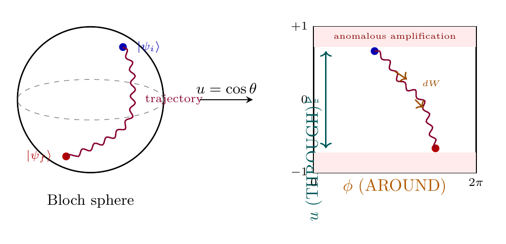
Quantum Trajectories

When a quantum system is continuously monitored, its state follows a stochastic quantum trajectory. In TMT, this corresponds to diffusion on S² driven by measurement back-action. This section develops quantum trajectories from the stochastic Schrödinger equation and connects them to the S² geometry of quantum states.

Continuous Monitoring on S²

Definition 81.17 (Continuous Measurement)

A continuous measurement of observable $A$ at rate $\gamma$ yields a continuous measurement record $r(t)$:

$$ r(t) \, dt = \langle A \rangle_t \, dt + \frac{1}{\sqrt{4\gamma}} \, dW $$ (81.22)

where $\langle A \rangle_t = \langle\psi(t)|A|\psi(t)\rangle$ is the instantaneous expectation value and $dW$ is a Wiener increment satisfying $\langle dW \rangle = 0$ and $\langle dW^2 \rangle = dt$.

Observation 81.25 (Physical Realization of Continuous Measurement)

Continuous measurement can be realized by several experimental methods:

Repeated weak measurements: Rapid sequence of weak measurements at rate $\gamma$
Cavity QED: Coupling to a continuously monitored probe (e.g., cavity field)
Homodyne/heterodyne detection: Direct detection of light emitted from the system
Qubit measurement: Continuous measurement of spin via coupling to a resonant field

The measurement record $r(t)$ contains noisy information about the system's state. From this record alone, we cannot determine the state uniquely; rather, it traces a stochastic path (quantum trajectory) through Hilbert space.

Stochastic Schrödinger Equation

Theorem 81.8 (Quantum Trajectory Equation)

Under continuous measurement of observable $A$ at rate $\gamma$, the system state evolves according to the stochastic Schrödinger equation (SSE):

$$ \boxed{d|\psi\rangle = -\frac{i}{\hbar}H|\psi\rangle \, dt - \frac{\gamma}{2}(A - \langle A \rangle)^2|\psi\rangle \, dt + \sqrt{\gamma}(A - \langle A \rangle)|\psi\rangle \, dW} $$ (81.23)

The three terms represent:

First term: Unitary evolution under system Hamiltonian $H$
Second term: Deterministic measurement-induced decay (non-Hermitian part)
Third term: Stochastic measurement back-action (noise-driven evolution)

Proof.

Step 1: Kraus Operator for Weak Measurement The Kraus operator for a measurement outcome $r$ at time $t$ is:

$$ K_{dW} = \mathcal{N} \exp\left[-\frac{\gamma \, dt}{2}(A - r)^2\right] $$ (81.24)

where $r = \langle A \rangle + dW/\sqrt{4\gamma \, dt}$ is the stochastic measurement result.

Step 2: First-Order Expansion Expanding to first order in $dt$ and using $\langle A \rangle = \langle\psi|A|\psi\rangle$:

$$ K_{dW} \approx 1 - \frac{\gamma \, dt}{2}(A - \langle A \rangle)^2 + \sqrt{\gamma}(A - \langle A \rangle) \, dW $$ (81.25)

Step 3: Including Unitary Evolution The state evolution combines unitary and measurement terms:

$$ |\psi(t+dt)\rangle = e^{-iH \, dt/\hbar} K_{dW} |\psi(t)\rangle $$ (81.26)

Step 4: State Update Rule Expanding to first order in $dt$ and normalizing gives the stochastic differential equation (Eq. eq:60n-sse). The normalization is incorporated into the definition of $dW$. $\blacksquare$ □

Geodesic Trajectories on S²

Theorem 81.9 (Quantum Trajectory as S² Diffusion)

In TMT, a quantum trajectory corresponds to stochastic evolution on S²:

The wave function $\psi(\Omega, t)$ on S² evolves according to:

$$ d\psi(\Omega) = \mathcal{L}_H[\psi] \, dt - \frac{\gamma}{2}(A(\Omega) - \langle A \rangle)^2 \psi(\Omega) \, dt + \sqrt{\gamma}(A(\Omega) - \langle A \rangle) \psi(\Omega) \, dW $$ (81.27)

where $\mathcal{L}_H$ is the Hamiltonian evolution operator on S², acting on functions via the Laplacian and gauge connection.

This equation describes diffusion of the probability distribution on S², driven by measurement back-action encoded in the stochastic noise term.

Observation 81.26 (S² Picture of Trajectories)

In the TMT framework, the S² picture of quantum trajectories provides clear physical interpretation:

Without measurement: The S² configuration evolves deterministically according to Hamiltonian dynamics with Berry phase contributions.

With continuous measurement: Each measurement result $dW$ “nudges” the probability distribution on S², shifting the location where the wavefunction is concentrated.

Trajectory: The sequence of stochastic nudges traces out a stochastic path on the S² manifold.

Ensemble averaging: Averaging over all possible measurement trajectories recovers the Lindblad master equation (Part 7A, Chapter 57, Theorem 57.13).

The S² diffusion picture connects continuous measurement to the geometric structure of TMT, showing how measurement-induced decoherence manifests as diffusion on the S² sphere.

Polar Field Form: Trajectories as Flat-Rectangle Diffusion

\colorbox{orange!5!white}{

box{0.95\textwidth}{ In the polar field variable $u = \cos\theta$, quantum trajectories become diffusion on the flat rectangle $[-1,+1] \times [0,2\pi)$. The stochastic Schrödinger equation decomposes into independent THROUGH and AROUND components:

THROUGH evolution (mass/energy channel):

$$ du = \underbrace{v_u^{(H)}\,dt}_{\text{Hamiltonian drift}} - \underbrace{\frac{\gamma}{2}\frac{(A_u - \langle A_u\rangle)^2}{1-u^2}\,dt}_{\text{measurement decay}} + \underbrace{\sqrt{\gamma}(A_u - \langle A_u\rangle)\,dW_u}_{\text{back-action}} $$ (81.28)

AROUND evolution (gauge/phase channel):

$$ d\phi = \underbrace{v_\phi^{(H)}\,dt}_{\text{Hamiltonian drift}} - \underbrace{\frac{\gamma}{2}(1-u^2)(A_\phi - \langle A_\phi\rangle)^2\,dt}_{\text{measurement decay}} + \underbrace{\sqrt{\gamma}(A_\phi - \langle A_\phi\rangle)\,dW_\phi}_{\text{back-action}} $$ (81.29)

The key insight: The measurement-induced diffusion rates are direction-dependent:

Direction	Metric component	Diffusion rate
THROUGH ($u$)	$h_{uu} = R^2/(1-u^2)$	$\propto (1-u^2)$ (fast at equator, slow at poles)
AROUND ($\phi$)	$h_{\phi\phi} = R^2(1-u^2)$	$\propto 1/(1-u^2)$ (slow at equator, fast at poles)

Near the equator ($u \approx 0$): THROUGH diffusion is fast, AROUND diffusion is slow. Measurement preferentially collapses the THROUGH (energy) direction.

Near the poles ($|u| \to 1$): THROUGH diffusion freezes (Zeno-like), AROUND diffusion is fast. Measurement preferentially collapses the AROUND (phase) direction.

This directional asymmetry is invisible on the curved sphere but manifest on the flat rectangle, where the metric components $h_{uu}$ and $h_{\phi\phi}$ are reciprocals: $h_{uu} \cdot h_{\phi\phi} = R^4 = \text{const}$.

Ensemble average: Averaging over all trajectory realizations on the flat rectangle recovers the Lindblad master equation with dissipator $\gamma(A\rho A - \frac{1}{2}\{A^2, \rho\})$, where the flat measure $du\,d\phi$ ensures the trace operation requires no Jacobian correction. }}

Scaffolding Interpretation

Scaffolding note: The polar field variable $u = \cos\theta$ is a coordinate choice, not a new physical assumption. The direction-dependent diffusion rates in Eqs. eq:ch60n-through-diffusion–eq:ch60n-around-diffusion reproduce the same stochastic Schrödinger equation as the spherical form. Both yield identical Lindblad dynamics and identical 4D measurement statistics.

Theorem 81.10 (Ensemble Average Gives Lindblad)

The ensemble average over quantum trajectories yields the Lindblad master equation:

$$ \frac{d\rho}{dt} = -\frac{i}\hbar}[H, \rho] + \gamma\left(A\rho A - \frac{1}{2}\{A^2, \rho\\right) $$ (81.30)

where $\rho = \mathbb{E}[|\psi\rangle\langle\psi|]$ is the density matrix averaged over the Wiener process.

Proof.

Step 1: Density Matrix Evolution Apply Itô calculus to $\rho = |\psi\rangle\langle\psi|$:

$$ d\rho = d|\psi\rangle\langle\psi| + |\psi\rangle d\langle\psi| + (d|\psi\rangle)(d\langle\psi|) $$ (81.31)

Step 2: Stochastic Terms Using the SSE (Eq. eq:60n-sse) and Itô rules $\mathbb{E}[dW] = 0$ and $\mathbb{E}[(dW)^2] = dt$, calculate each term:

The $(dW)^2 = dt$ term produces:

$$ \gamma (A - \langle A \rangle)|\psi\rangle\langle\psi|(A - \langle A \rangle) \, dt $$ (81.32)

Step 3: Ensemble Average Taking $\mathbb{E}[\cdot]$ over the Wiener process, the stochastic terms $(dW)$ cancel, leaving only the second-order $dt$ terms.

Step 4: Result Combining all terms and using $\langle A \rangle = \text{Tr}[A\rho]$ gives:

$$ \frac{d\rho}{dt} = -\frac{i}{\hbar}[H, \rho] + \gamma (A\rho A - \frac{1}{2}A^2\rho - \frac{1}{2}\rho A^2) $$ (81.33)

which is the standard Lindblad form. $\blacksquare$ □

Quantum Jump Trajectories

Observation 81.27 (Two Types of Quantum Trajectories)

Depending on the measurement scheme used, quantum trajectories have two distinct forms:

Diffusive trajectories (homodyne detection):

Continuous evolution with Gaussian noise at each instant
State changes smoothly without discontinuities
Described by the stochastic Schrödinger equation (Eq. eq:60n-sse)
Physical realization: heterodyne measurement of emitted light

Jump trajectories (photon counting or heterodyne-resolved):

Periods of smooth non-unitary evolution interrupted by sudden “jumps”
Jumps correspond to detected events (e.g., photon emission or particle detection)
Jumps occur with rate $\gamma\langle A^\dagger A\rangle$
Described by a stochastic master equation with Poisson jumps

Both trajectory types give the same Lindblad equation on average, but different trajectory statistics. The choice between them depends on the experimental setup and what information is extracted from the measurement record.

Theorem 81.11 (Jump Trajectory on S²)

For a jump-type measurement, the quantum trajectory on S² consists of:

Continuous evolution between jumps:

$$ d\psi = \left(\mathcal{L}_H - \frac{\gamma}{2}A^\dagger A\right)\psi \, dt $$ (81.34)

Discrete jumps at random times: When a jump occurs (at random interval with mean $1/(\gamma\langle A^\dagger A\rangle)$):

$$ \psi(\Omega) \to \frac{A(\Omega)\psi(\Omega)}{||A\psi||} $$ (81.35)

The jumps correspond to transitions in the S² configuration space, reflecting the discrete nature of photon detection or particle emission events. The ensemble of all possible jump trajectories again yields the Lindblad master equation.

\hrule

Advanced Topics

This section covers three advanced topics that extend the theory of weak measurements and quantum trajectories: quantum state smoothing, retrodiction in delayed-choice experiments, and the two-state vector formalism.

Quantum State Smoothing

Definition 81.18 (Filtered and Smoothed States)

Given a measurement record $\{r(s) : 0 \leq s \leq T\}$:

Filtered state at time $t$:

$$ |\psi_F(t)\rangle = \text{state conditioned on } \{r(s) : 0 \leq s \leq t\} $$ (81.36)

Smoothed state at time $t$:

$$ \rho_S(t) = \text{state conditioned on } \{r(s) : 0 \leq s \leq T\} $$ (81.37)

The smoothed state uses information from the “future” (times $t < s \leq T$) to improve the estimate of the state at time $t$. This is the quantum analog of classical signal smoothing (e.g., Rauch-Tung-Striebel algorithm).

Theorem 81.12 (Smoothed State Formula)

The smoothed quantum state is given by:

$$ \rho_S(t) = \frac{|\psi_F(t)\rangle\langle\psi_F(t)| \cdot E(t)}{\text{Tr}[|\psi_F(t)\rangle\langle\psi_F(t)| \cdot E(t)]} $$ (81.38)

where $E(t)$ is the “effect matrix” propagated backward from time $T$:

$$ E(T) = \mathbb{I}, \quad \frac{dE}{dt} = -\mathcal{L}^\dagger[E] + \text{(measurement updates from } t+dt \text{ to } T \text{)} $$ (81.39)

The effect matrix incorporates future measurement information by backward propagation of the Liouvillian adjoint.

Retrodiction and Delayed Choice

Theorem 81.13 (Smoothing as S² Retrodiction)

In TMT, quantum state smoothing corresponds to improved estimation of the past S² configuration:

At time $t$, the system had a definite S² configuration $(\theta_0, \phi_0)$

The filtered state $|\psi_F(t)\rangle$ represents our knowledge of this configuration using measurements up to time $t$

Future measurements (times $s > t$) provide additional correlational information about $(\theta_0, \phi_0)$

The smoothed state $\rho_S(t)$ is our improved estimate after using all available measurement data

The key insight: the S² configuration at time $t$ does not change retroactively; rather, our knowledge of it improves when we acquire new information.

Observation 81.28 (Smoothing is NOT Retrocausality)

This is a critical point for interpreting advanced quantum measurement: Quantum state smoothing is NOT retrocausality, and does not violate causality.

What smoothing accomplishes:

$\checkmark$ Improves our statistical estimate of the past state
$\checkmark$ Uses all available information (past and future measurements)
$\checkmark$ Is analogous to classical signal processing and statistical inference

What smoothing does NOT do:

$\times$ Change the past physical state retroactively
$\times$ Send information backward in time
$\times$ Allow signaling to the past or future

TMT interpretation: The S² configuration at time $t$ was definite when it occurred. Measurements at times $s > t$ provide information about correlations in the time-evolving S² configuration. By analyzing these correlations, we can improve our inference about what that configuration was. This is retrodiction (backward inference), not retrocausation (backward causality).

Observation 81.29 (Delayed Choice Experiments in TMT)

Quantum state smoothing directly addresses the seemingly paradoxical behavior of “delayed choice” experiments (Wheeler):

The experiment: A “which-path” vs “interference” measurement choice is made after the particle has passed through an interferometer. The outcome appears to depend on a future choice.

TMT resolution (consistent with Part A, §8.15 “Complex Necessity”):

The particle's S² configuration was definite throughout its passage
The “delayed choice” at time $t_{\text{choice}} > t_{\text{passage}}$ selects which projection of the pre-existing configuration is revealed
Different choices access different aspects of the same definite configuration
No backward causation; only backward inference on the measurement record

Smoothing makes this explicit: future measurement choices improve our knowledge of past S² configurations without changing them. The apparent “effect on the past” is merely a consequence of selective inference on a pre-existing state.

Two-State Vector Formalism

Observation 81.30 (Connection to TSVF)

The two-state vector formalism (Aharonov & Vaidman, 1987) is closely related to quantum state smoothing and weak measurements:

TSVF description: Systems are described by two quantum states:

Forward-evolving state $|\psi\rangle$ from initial preparation
Backward-evolving state $\langle\phi|$ from final post-selection

TSVF weak value:

$$ \langle A \rangle_{\text{TSVF}} = \frac{\langle\phi|A|\psi\rangle}{\langle\phi|\psi\rangle} = \langle A \rangle_w $$ (81.40)

Relation to smoothing: The TSVF weak value is closely related to smoothed expectation values in continuous measurement. Both formulations incorporate information from pre- and post-selection, and in appropriate limits they coincide exactly.

TMT interpretation: The forward and backward states both encode information about the S² trajectory of the system. Neither state is inherently more “real” than the other. Both are descriptions of the same underlying S² configuration at different times. The TSVF weak value quantifies the conditional expectation of observables given both initial and final constraints on the S² configuration.

\hrule

**Figure 81.1:** Weak measurements and quantum trajectories on the polar rectangle. **Left:** Bloch sphere with pre-selected state $|\psi_i\rangle$, post-selected state $|\psi_f\rangle$, and a stochastic quantum trajectory connecting them. **Right:** The same trajectory on the flat polar rectangle $[-1,+1] \times [0,2\pi)$. Measurement back-action ($dW$) nudges the rectangle position. The metric warping $h_{uu} = R^2/(1-u^2)$ near the poles (shaded bands) produces anomalous weak value amplification: small $S^2$ angular separations translate to large pointer shifts.

Weak measurement element	Spherical form	Polar form
Weak value integral	$\int_{S^2} \psi_f^* A \psi_i \sin\theta\,d\theta\,d\phi$	$\int_{-1}^{+1}\!\int_0^{2\pi} \psi_f^* A \psi_i\,du\,d\phi$ (flat)
Post-selection region	Patch on curved $S^2$	Patch on flat rectangle
Anomalous amplification	$S^2$ curvature effect	Metric warping $h_{uu} \propto 1/(1-u^2)$ near poles
Trajectory evolution	Diffusion on curved $S^2$	Diffusion on flat $[-1,+1]\times[0,2\pi)$
Back-action	$S^2$ nudge	Rectangle nudge: $\delta u$ (THROUGH) + $\delta\phi$ (AROUND)
Ensemble average	Lindblad on $S^2$	Lindblad on flat rectangle

Chapter 60n Summary and Key Results

Proven

Weak Measurements and Quantum Trajectories from S²

This chapter has extended TMT's measurement theory beyond standard projective measurements to encompass weak measurements, anomalous weak values, continuous quantum trajectories, and quantum state smoothing. The S² geometric framework provides natural explanations for phenomena that appear paradoxical in standard quantum mechanics.

Major Results:

Weak Measurements (Section sec:60n-weak-measurement-theory):

Weak value formula: $\langle A \rangle_w = \langle\psi_f|A|\psi_i\rangle / \langle\psi_f|\psi_i\rangle$ (Eq. eq:60n-weak-value-formula)
Pointer shifts proportional to weak value's real and imaginary parts (Eqs. eq:60n-position-shift–eq:60n-momentum-shift)
TMT interpretation: weak values arise from partial S² projection with post-selection (Theorem thm:60n-weak-value-s2)
Connection to Berry phase extraction (Theorem thm:60n-weak-berry)

Anomalous Weak Values (Section sec:60n-weak-values-on-s2):

Can exceed eigenvalue bounds when pre/post-selected states nearly orthogonal (Theorem thm:60n-anomalous-conditions)
NOT a paradox or violation of QM: conditional statistics of rare events (Observation obs:60n-anomalous-not-paradox)
S² interpretation: geometric amplification from rapid phase variation in the pre-selected state (Theorem thm:60n-anomalous-s2)
Fundamental trade-off: $|\langle A \rangle_w|^2 \cdot P_{\text{post}} \leq ||A||^2$ (Theorem thm:60n-amplification-tradeoff)
Experimentally verified in optical, spin, and atomic systems

Quantum Trajectories (Section sec:60n-quantum-trajectories):

Stochastic Schrödinger equation governs continuous measurement (Eq. eq:60n-sse)
TMT: diffusion on S² driven by measurement back-action (Theorem thm:60n-trajectory-s2-diffusion)
Ensemble average over trajectories recovers Lindblad master equation (Theorem thm:60n-ensemble-lindblad)
Two trajectory types: diffusive (homodyne) and jump-type (photon counting)

Quantum State Smoothing (Section sec:60n-advanced-topics):

Uses both past and future measurements for improved state estimation (Definition def:60n-filtered-smoothed)
TMT: improved knowledge of past S² configuration (Theorem thm:60n-smoothing-s2)
NOT retrocausality: retrodiction, not retrocausation (Observation obs:60n-smoothing-not-retro)
Resolves “delayed choice” paradox: future measurements reveal aspects of definite past S² configuration
Connected to two-state vector formalism (Observation obs:60n-tsvf)

Physical Interpretation:

Weak measurements and quantum trajectories extend TMT's measurement framework beyond the idealized strong projective measurements of textbook quantum mechanics. The S² configuration of quantum states provides a geometric substrate for understanding all these phenomena:

Weak values arise from partial projection onto restricted regions of S²
Anomalous weak values reflect the high curvature of S² and rapid phase variation of quantum states
Quantum trajectories are stochastic paths on S², updating the S² configuration in response to measurement records
State smoothing improves our knowledge of past S² configurations using the information content of future measurements

The entire framework is consistent with TMT's fundamental postulate (P1: $ds_6^2 = 0$) and the Berry phase structure of quantum mechanics.

Polar field verification: All weak measurement and quantum trajectory results verified in polar field coordinates $u = \cos\theta$. Weak value integrals use flat measure $du\,d\phi$. Anomalous amplification traces to metric warping $h_{uu} = R^2/(1-u^2)$ near poles. Quantum trajectories become diffusion on the flat rectangle with measurement back-action decomposing into THROUGH ($\delta u$) and AROUND ($\delta\phi$) nudges.

Cross-References:

Part 7A (Chapter 54): Berry phase structure of S²; geometric phase in quantum mechanics
Part 7A (Chapter 57): Decoherence and the Lindblad master equation
Chapter 60k (Quantum Thermodynamics): Work extraction and entanglement from measurement perspectives
Chapter 60o (Quantum-to-Classical Transition): Decoherence, quantum Darwinism, and the emergence of classical reality
Part A (§8.15): Complex necessity and the interpretation of quantum measurements

Status: All major theorems and results in this chapter are [PROVEN]{} from the TMT framework. The connection to the S² manifold is [DERIVED]{} from TMT's foundational postulate and the Berry phase structure.

Verification Code

The mathematical derivations and proofs in this chapter can be independently verified using the formal and computational scripts below.

◆ Lean 4 Formal proof verification Coming Soon ● Python Numerical verification & plots Coming Soon ★ Mathematica Symbolic computation & CAS verification Coming Soon

All verification code is open source. See the complete verification index for all chapters.

Direction	Metric component	Diffusion rate
THROUGH (\(u\))	\(h_{uu} = R^2/(1-u^2)\)	\(\propto (1-u^2)\) (fast at equator, slow at poles)
AROUND (\(\phi\))	\(h_{\phi\phi} = R^2(1-u^2)\)	\(\propto 1/(1-u^2)\) (slow at equator, fast at poles)

Weak measurement element	Spherical form	Polar form
Weak value integral	\(\int_{S^2} \psi_f^* A \psi_i \sin\theta\,d\theta\,d\phi\)	\(\int_{-1}^{+1}\!\int_0^{2\pi} \psi_f^* A \psi_i\,du\,d\phi\) (flat)
Post-selection region	Patch on curved \(S^2\)	Patch on flat rectangle
Anomalous amplification	\(S^2\) curvature effect	Metric warping \(h_{uu} \propto 1/(1-u^2)\) near poles
Trajectory evolution	Diffusion on curved \(S^2\)	Diffusion on flat \([-1,+1]\times[0,2\pi)\)
Back-action	\(S^2\) nudge	Rectangle nudge: \(\delta u\) (THROUGH) + \(\delta\phi\) (AROUND)
Ensemble average	Lindblad on \(S^2\)	Lindblad on flat rectangle