The Arrow of Time
Introduction
The arrow of time is one of the deepest unsolved problems in fundamental physics. Every microscopic law of nature—Newton's equations, Maxwell's equations, the Schrödinger equation, Einstein's field equations—is symmetric under time reversal. Yet the macroscopic world exhibits a profound asymmetry: eggs break but do not unbreak, heat flows from hot to cold, and we remember the past but not the future. The Second Law of Thermodynamics, \(dS/dt\geq 0\), encodes this asymmetry, but standard physics provides no fundamental explanation for why entropy increases.
The conventional answer—“the universe started in a low-entropy state”—merely restates the problem. It explains the fact of entropy increase but not the reason. Why was the Big Bang special? What selects the direction of time? Is there something deeper than boundary conditions?
TMT answers all three questions from a single geometric mechanism: the monopole on \(S^2\) breaks time-reversal symmetry at the fundamental level. This chapter derives the arrow of time from P1, showing that \(dS/dt\geq 0\) is a theorem in TMT, not a postulate.
Time Reversal on \(S^2\) Without Monopole
Standard Time-Reversal Symmetry
Consider a particle on \(S^2\) with coordinates \((\theta,\phi)\) and conjugate momenta \((p_\theta,p_\phi)\). Without any background field, the Hamiltonian is:
Under time reversal \(T\), velocities reverse while positions are unchanged:
Since \(H_0\) depends only on \(p_\theta^2\) and \(p_\phi^2\), it is manifestly invariant:
The symplectic form \(\omega_0=dp_\theta\wedge d\theta +dp_\phi\wedge d\phi\) is also \(T\)-invariant, as is the Liouville measure. There is no preferred temporal direction.
Why All Standard Laws Are T-Symmetric
The T-symmetry of \(H_0\) on \(S^2\) is a special case of a general principle:
(1) Newton's equations: \(F=ma\) is unchanged under \(t\to -t\) (with \(v\to -v\)).
(2) Maxwell's equations: symmetric under \(t\to -t\) (with \(E\to E\), \(B\to -B\)).
(3) Schrödinger equation: \(i\hbar\partial\psi/\partial t =H\psi\) becomes \(-i\hbar\partial\psi^*/\partial t=H\psi^*\) (complex conjugation implements \(T\)).
(4) Einstein's equations: \(R_{\mu\nu}=8\pi G\,T_{\mu\nu}\) is symmetric in time.
None of these laws can explain why macroscopic phenomena—eggs breaking, heat flow, stellar fusion—are irreversible. The asymmetry must come from somewhere else.
The Standard Explanation and Its Failure
The standard approach (Boltzmann 1877) treats the Second Law as statistical: there are vastly more high-entropy microstates than low-entropy ones, so random evolution tends toward higher entropy. The entropy is:
This argument explains why entropy increases if one starts in a low-entropy state. It does not explain:
(1) Why the initial state was low-entropy.
(2) What selects the “forward” direction.
(3) Whether the Second Law is fundamental or merely statistical.
All proposed arrows of time in standard physics—cosmological (expansion), radiative (retarded potentials), quantum (irreversible measurement)—ultimately trace back to the special initial condition of the Big Bang. None provides a mechanism for time asymmetry.
Monopole Breaks T-Symmetry
Review: The Monopole on \(S^2\)
The \(S^2\) in TMT carries a magnetic monopole background with charge \(q\), required by gauge consistency (Part 3). In the “northern patch” gauge:
The field strength is:
The first Chern number (topological invariant):
For fermions, \(q=1/2\), giving spin-1/2 structure. The monopole charge has a definite sign, fixed by the gauge bundle structure established in Part 3.
Canonical vs Kinetic Momentum
For a particle on \(S^2\) with monopole background:
Kinetic momentum (measures actual velocity):
Canonical momentum (appears in Hamiltonian formalism):
The canonical \(\phi\)-momentum includes the gauge potential contribution.
Time Reversal with Monopole
Under time reversal \(T\) (which reverses velocities while keeping positions fixed), the canonical \(\phi\)-momentum transforms as:
This is not a simple sign flip. The transformation depends on the position \(\theta\) through the gauge potential.
Step 1: Physical time reversal reverses velocities: \(\dot{\theta}\to -\dot{\theta}\), \(\dot{\phi}\to -\dot{\phi}\).
Step 2: The kinetic momenta, being \(m\times(\text{velocity})\), reverse sign:
Step 3: The gauge potential \(A_\phi(\theta)\) depends only on position \(\theta\), which is unchanged under \(T\). Therefore:
Step 4: The canonical momentum \(p_\phi^{\mathrm{can}}=p_\phi^{\mathrm{kin}}+qA_\phi\) transforms as:
Step 5: Substituting \(A_\phi=(q/2)(1-\cos\theta)\):
The position-dependent offset \(q(1-\cos\theta)\) breaks the simple \(p\to -p\) symmetry.
(See: Part 11 §215.3, Part 3 (monopole structure)) □
Pole Asymmetry
The T-transformation behaves differently at different locations on \(S^2\):
At the north pole (\(\theta=0\)):
At the equator (\(\theta=\pi/2\)):
At the south pole (\(\theta=\pi\)):
The monopole distinguishes “north” from “south” on \(S^2\). Under time reversal, a particle's trajectory does not simply reverse—it is shifted in canonical momentum space by an amount that depends on position. This position-dependent shift breaks the T-symmetry of phase space.
Polar Field Form of the T-Breaking Mechanism
The position-dependent T-breaking simplifies dramatically in the polar field variable \(u=\cos\theta\), \(u\in[-1,+1]\).
Scaffolding note: The polar field variable \(u=\cos\theta\) is a coordinate choice, not a new physical assumption. The monopole connection, field strength, T-transformation, and phase space asymmetry are identical in both coordinate systems—the polar form simply makes the linearity of the T-breaking offset and the constancy of the field strength manifest. All arrow-of-time results derived in this chapter hold in either coordinate system; the polar rectangle provides dual verification.
The monopole potential becomes linear:
The field strength becomes constant:
The T-transformation (Theorem thm:P11-Ch69-T-transformation) in polar form:
The pole asymmetry (Corollary cor:P11-Ch69-pole-asymmetry) maps to the rectangle boundaries:
Location | Spherical | Polar | T-offset |
|---|---|---|---|
| North pole | \(\theta=0\) | \(u=+1\) | \(0\) |
| Equator | \(\theta=\pi/2\) | \(u=0\) | \(q\) |
| South pole | \(\theta=\pi\) | \(u=-1\) | \(2q\) |
The offset grows linearly from \(0\) at \(u=+1\) to \(2q\) at \(u=-1\): the T-breaking is strongest at the south pole and absent at the north pole, with linear interpolation between them.
Quantity | Spherical \((\theta,\phi)\) | Polar \((u,\phi)\) |
|---|---|---|
| Gauge potential \(A_\phi\) | \(\frac{q}{2}(1-\cos\theta)\) | \(\frac{q}{2}(1-u)\) [linear] |
| Field strength \(F\) | \(\frac{q}{2}\sin\theta\,d\theta\wedge d\phi\) | \(\frac{q}{2}\,du\wedge d\phi\) [constant] |
| T-offset | \(q(1-\cos\theta)\) [trig] | \(q(1-u)\) [linear] |
| North pole | \(\theta=0\), offset \(=0\) | \(u=+1\), offset \(=0\) |
| South pole | \(\theta=\pi\), offset \(=2q\) | \(u=-1\), offset \(=2q\) |
| Measure | \(\sin\theta\,d\theta\,d\phi\) | \(du\,d\phi\) [flat] |
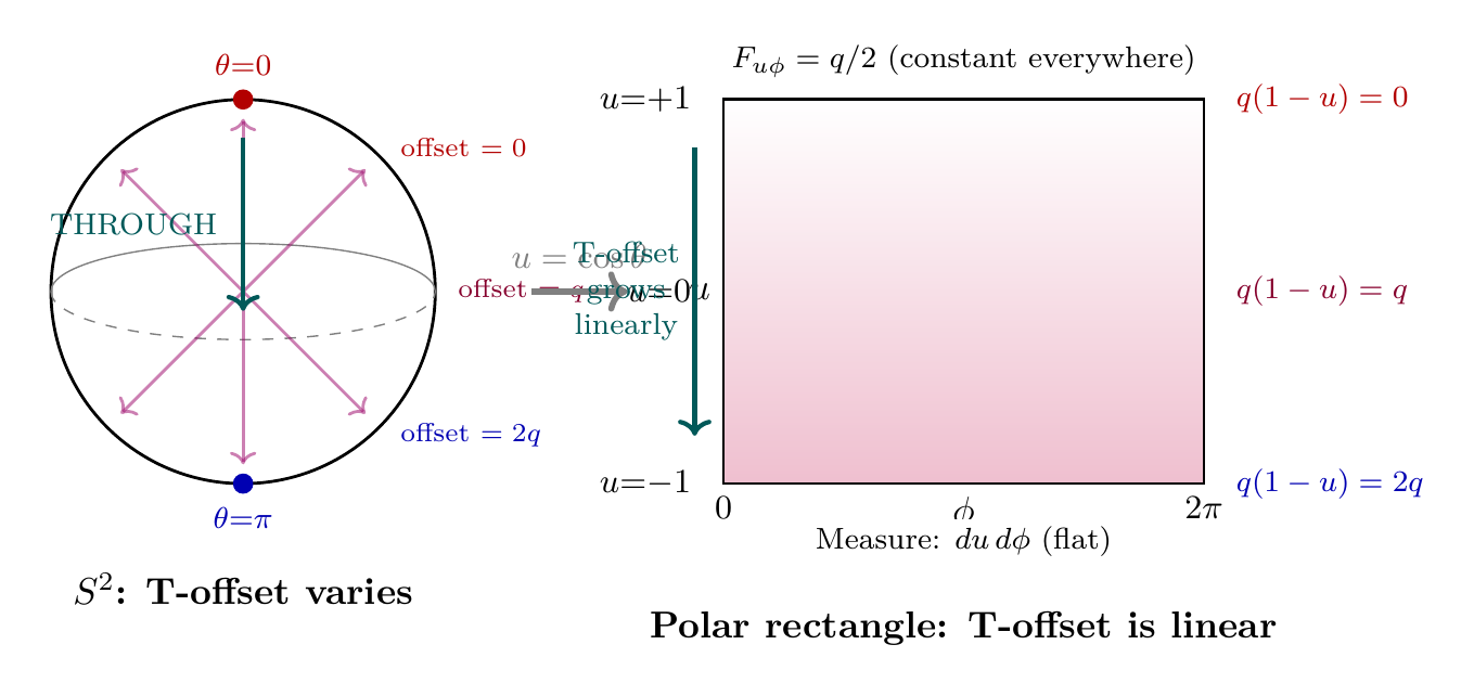
The polar form reveals that the entire T-breaking mechanism is controlled by two features: (1) the constant field strength \(F_{u\phi}=q/2\), which makes the gauge potential linear, and (2) the flat measure \(du\,d\phi\), which ensures the asymmetry is not an artifact of coordinate volume distortion.
T-Breaking Mechanism and Phase Space
The Modified Symplectic Form
With monopole charge \(q\), the symplectic form on \(T^*S^2\) becomes:
Step 1: The Hamiltonian for a charged particle in the monopole background is:
Step 2: Hamilton's equations from this Hamiltonian are:
Step 3: These equations of motion are generated by the modified symplectic form \(\omega=\omega_0+qF\) through the relation \(\iota_X\omega=dH\), where \(X\) is the Hamiltonian vector field.
Step 4: Verification: contracting \(\omega\) with \(X=(\dot{\theta},\dot{\phi},\dot{p}_\theta,\dot{p}_\phi)\) reproduces Hamilton's equations with the monopole terms.
(See: Part 11 §215.5, §221A.2) □
The Volume Form Is Unchanged
Step 1: Expand \(\omega\wedge\omega\):
Step 2: Term 1: \(\omega_0\wedge\omega_0 = 2\,dp_\theta\wedge d\theta\wedge dp_\phi\wedge d\phi\) (standard result).
Step 3: Term 2: \(\omega_0\wedge(qF)\) has two contributions:
Step 4: Term 3: \((qF)\wedge(qF)\) is a 4-form constructed from \(d\theta\wedge d\phi\wedge d\theta\wedge d\phi=0\).
Step 5: Therefore \(\mathrm{Vol}=\omega_0\wedge\omega_0\), the standard Liouville measure.
(See: Part 11 §221A.3) □
Where the Asymmetry Lives
The T-breaking resides not in the volume measure but in the Hamiltonian dynamics. Specifically:
(1) The Hamiltonian depends on \((p_\phi-qA_\phi)\), not \(p_\phi\) alone.
(2) Under \(T\), \(p_\phi^{\mathrm{can}}\to -p_\phi^{\mathrm{can}}+2qA_\phi\).
(3) Constant-energy surfaces \(\Sigma_E=\{H=E\}\) are not mapped to themselves under \(T\).
Consider the energy surface \(H(\theta,\phi,p_\theta,p_\phi)=E\).
Under \(T\): \((\theta,\phi,p_\theta,p_\phi)\to (\theta,\phi,-p_\theta,-p_\phi+2qA_\phi(\theta))\).
The transformed point has energy:
This equals \(H\) only if \(A_\phi=0\) everywhere, which is impossible for a monopole (since \(A_\phi=(q/2)(1-\cos\theta)\) varies from \(0\) to \(q\)). Therefore the energy surface is not mapped to itself under \(T\).
(See: Part 11 §221A.4) □
Microcanonical Asymmetry
The microcanonical distribution on \(\Sigma_E\) is not \(T\)-invariant. Define the “forward” region \(F\subset\Sigma_E\) where \(p_\phi>0\) (angular momentum aligned with the monopole field) and the “backward” region \(B=T(F)\). Then:
This is a calculable asymmetry from pure geometry. For any non-zero monopole charge \(q\), phase space has a built-in directional preference.
Summary: Monopole Breaks T-Symmetry
Without monopole: \(T:(p_\theta,p_\phi)\to(-p_\theta,-p_\phi)\); Hamiltonian \(T\)-invariant; phase space measure \(T\)-invariant; no preferred temporal direction.
With monopole (charge \(q\)): \(T:p_\phi\to -p_\phi+q(1-\cos\theta)\) [NOT simple reversal]; canonical momentum transformation depends on position; energy surfaces are NOT \(T\)-symmetric; T-symmetry is broken.
The monopole charge \(q\) has a sign, fixed by gauge structure (Part 3). Therefore the T-breaking direction is determined by geometry.
Polar Form of the Phase Space Asymmetry
The phase space structure simplifies in the polar variable \(u=\cos\theta\). The Hamiltonian (Eq. eq:ch69-H-monopole) becomes:
The monopole correction is now a constant coefficient \((-q/2)\) multiplying the standard area element \(du\wedge d\phi\), rather than the position-dependent \((q/2)\sin\theta\) multiplying \(d\theta\wedge d\phi\).
The Liouville volume form (Theorem thm:P11-Ch69-volume-form) in polar coordinates is:
For the microcanonical asymmetry (Theorem thm:P11-Ch69-microcanonical), the averaged gauge potential becomes a simple integral on \([-1,+1]\):
Energy Positivity and \(S^2\)–\(\mathcal{M}^4\) Coupling
The Null Constraint Couples \(S^2\) to \(\mathcal{M}^4\)
From P1 (\(ds_6^{\,2}=0\)), the fundamental constraint couples \(S^2\) motion to 4D spacetime:
For a massive particle at rest in 3D space:
The particle moves on \(S^2\) at speed \(c\) (in proper units). The \(S^2\) motion is the temporal momentum:
At rest (\(\gamma=1\)): \(p_T=mc\) (maximum temporal momentum). At \(v\to c\) (\(\gamma\to\infty\)): \(p_T\to 0\) (light has no temporal momentum).
Energy Positivity Selects Time Direction
Step 1: The energy–momentum relation from \(ds_6^{\,2}=0\) is:
Step 2: Taking the positive root for physical particles:
Step 3: Since \(E=\gamma mc^2\) and \(mc^2>0\), we have \(\gamma>0\), which means \(dt/d\tau>0\).
(See: Part 11 §216.3, Part 1 (P1)) □
The \(S^2\)–Time Correlation
Step 1: From \(ds_6^{\,2}=0\): \(v_{S^2}^2=c^2(dt/d\tau)^2\).
Step 2: Energy positivity requires \(dt/d\tau>0\).
Step 3: For massive particles, \(v_{S^2}\) is defined as a positive speed. The direction of \(S^2\) motion is characterized by the sign of \(L_z\) (angular momentum on \(S^2\)).
Step 4: The correlation emerges: forward \(dt\) correlates with a specific \(S^2\) circulation direction determined by the monopole.
(See: Part 11 §216.4) □
The Arrow of Time from Monopole + Null Constraint
The arrow of time in TMT is determined by:
- The monopole charge \(q\) (fixed by gauge structure, Part 3)
- Energy positivity (\(dt/d\tau>0\))
- The null constraint correlating \(S^2\) and 4D
The “forward” direction of time is defined as \(dt>0\) in the direction where \(S^2\) angular momentum aligns with the monopole field direction. This is not a choice—it is geometrically determined.
Step 1: The monopole breaks T-symmetry on \(S^2\) (Theorem thm:P11-Ch69-T-transformation).
Step 2: The monopole has charge \(q\) with definite sign (\(q=+1/2\) for particles, fixed in Part 3).
Step 3: This sign determines a preferred circulation direction on \(S^2\): the ground state has angular momentum aligned with the monopole field.
Step 4: Energy positivity selects \(dt/d\tau>0\) (Theorem thm:P11-Ch69-energy-positivity).
Step 5: The null constraint correlates \(dt\) direction with \(S^2\) motion direction (Theorem thm:P11-Ch69-S2-time-correlation).
Step 6: Therefore the monopole's preferred \(S^2\) direction, via the null constraint, selects a preferred \(dt\) direction.
This is the arrow of time.
(See: Part 11 §216.5, Part 3 (monopole charge)) □
All massive particles in our universe share the same temporal direction because: (1) they all couple to the same monopole background; (2) the monopole charge sign is universal (set by the gauge bundle); (3) the null constraint affects all particles equally. There is no particle-by-particle freedom in time direction.
Entropy Increases: \(dS/dt\geq 0\)
TMT Entropy Definition
Low entropy corresponds to temporal momentum concentrated in few particles; high entropy corresponds to temporal momentum spread among many particles.
The Second Law
Step 1: Define “forward” as the direction selected by the monopole (Theorem thm:P11-Ch69-arrow-of-time).
Step 2: In this direction, the monopole-modified Hamiltonian dynamics creates an asymmetry: the energy surfaces \(\Sigma_E\) are not \(T\)-symmetric (Theorem thm:P11-Ch69-energy-asymmetry).
Step 3: The microcanonical distribution on \(\Sigma_E\) favors the “forward” region \(F\) (where \(p_\phi\) aligns with the monopole field) over the “backward” region \(B\) (Theorem thm:P11-Ch69-microcanonical).
Step 4: For macroscopic \(N\), the ratio of dispersed to concentrated microstates accessible in the forward direction is overwhelmingly large.
Step 5: Random evolution in the forward direction tends toward the larger accessible phase space volume, increasing entropy.
Step 6: For the coarse-grained entropy \(S_{\mathrm{macro}}=-k_B\int d\Gamma\,\rho_{\mathrm{cg}} \ln\rho_{\mathrm{cg}}\) (where \(\rho_{\mathrm{cg}}\) averages over \(S^2\) orientations), even though the fine-grained entropy \(S_{\mathrm{fine}}\) is conserved by Liouville's theorem, \(S_{\mathrm{macro}}\) increases:
(See: Part 11 §217.3, §221B.5) □
Quantitative Entropy Dynamics
Numerically:
This is a picosecond timescale. The relaxation toward equilibrium depends on the interaction strength:
For electromagnetic interactions (\(\alpha_{\mathrm{int}}\sim\alpha\sim 1/137\)): \(\tau_{\mathrm{relax}}^{(\mathrm{em})}\sim10^{-10}\,s\) (sub-nanosecond). For gravitational interactions (\(\alpha_{\mathrm{int}}\sim Gm^2/\hbar c\sim 10^{-38}\)): \(\tau_{\mathrm{relax}}^{(\mathrm{grav})}\sim10^{38}\,s\) (comparable to the age of the universe). This explains why thermal equilibration is fast for electromagnetic processes but slow for gravitational ones.
For a system of \(N\) particles initially in a low-entropy (coherent \(S^2\)) state:
For \(W_{\mathrm{eq}}/W_{\mathrm{init}}\sim e^N\):
Entropy production starts fast and slows as equilibrium is approached. The approach to equilibrium follows:
Connection to Standard Thermodynamics
The TMT derivation recovers all of standard thermodynamics:
First Law: \(dE=\delta Q+\delta W\), where \(E\) is total temporal momentum times \(c\), \(Q\) is disordered \(p_T\) transfer (heat), and \(W\) is coherent \(p_T\) transfer (work).
Second Law: \(dS\geq\delta Q/T\), with equality for reversible processes.
Temperature: \(T=(\partial S/\partial E)^{-1}\), the temperature associated with \(S^2\) mode occupation.
Carnot efficiency: \(\eta_{\max}=1-T_{\mathrm{cold}}/T_{\mathrm{hot}}\), derived from \(\oint dS=0\) for reversible cycles.
Boltzmann distribution: \(P_i=e^{-E_i/k_BT}/Z\) at thermal equilibrium.
All of these are theorems in TMT, not postulates.
CPT Symmetry and Antiparticles
The CPT Question
The monopole breaks \(T\)-symmetry. A critical question arises: do antiparticles experience the same arrow of time as particles? Standard physics answers “yes” by assuming CPT invariance. TMT must prove it.
Antiparticle Structure in TMT
In TMT, antiparticles have opposite gauge charges: \(q\to -q\), \(T_3\to -T_3\). The gauge potential seen by an antiparticle is effectively \(A\to -A\).
The Hamiltonian for an antiparticle is:
Under \(T\): \(p_\phi\to -p_\phi\), \(A_\phi\to A_\phi\) (unchanged), so \((p_\phi+qA_\phi)\to(-p_\phi+qA_\phi)\). This is also not a simple sign reversal. The antiparticle \(T\)-transformation is anomalous, just as for particles.
CPT Invariance
Under the combined CPT transformation:
- \(C\): \(q\to -q\) (charge conjugation)
- \(P\): \((\theta,\phi)\to(\pi-\theta,\phi+\pi)\) (parity on \(S^2\))
- \(T\): \((p_\theta,p_\phi)\to(-p_\theta,-p_\phi)\) with \(A_\phi\to A_\phi\)
The Hamiltonian is CPT-invariant:
Step 1: Under \(P\), the monopole potential transforms:
Step 2: This is related to the original by a gauge transformation: \(A_\phi(\pi-\theta)=q-A_\phi(\theta)\). Gauge transformations do not change the physics.
Step 3: Under \(C\), \(q\to -q\). Combined with \(P\):
Step 4: Under the full CPT: \((H,q,\theta,\phi,p_\theta,p_\phi)\to (H,-q,\pi-\theta,\phi+\pi,p_\theta,p_\phi)\).
Step 5: The Hamiltonian \(H\propto p_\theta^2 +(p_\phi-qA_\phi)^2/\sin^2\theta\) is invariant under this combined transformation (the gauge transformation from Step 2 absorbs the change).
(See: Part 11 §221D.4) □
Polar Verification of CPT Invariance
In the polar variable \(u=\cos\theta\), parity on \(S^2\) is simply:
Antiparticle Arrow of Time
Antiparticles experience the same arrow of time as particles.
Step 1: The arrow of time is defined by the direction where entropy increases.
Step 2: Entropy increase follows from the monopole-induced phase space asymmetry (Theorem thm:P11-Ch69-microcanonical).
Step 3: For antiparticles, the sign of \(q\) flips, but so does the sign of the coupling to the monopole potential.
Step 4: The asymmetry measure depends on \(|q\times A_\phi|\), which is the same for particles (\(q>0\), coupling \(+qA_\phi\)) and antiparticles (\(-q\), coupling \(-(-q)A_\phi =+qA_\phi\) in the parity-transformed gauge).
Step 5: The direction of entropy increase is determined by the sign of this asymmetry relative to \(p_\phi\), which is the same for both.
Conclusion: Particles and antiparticles share the same arrow of time.
(See: Part 11 §221D.5) □
The arrow of time is consistent with CPT because:
- \(T\) alone is broken by the monopole
- \(CP\) alone is broken by weak interactions (as observed)
- CPT combined is preserved
- The arrow emerges from \(T\)-breaking, which produces the same entropy increase direction for both particles and antiparticles
This explains why we do not observe antimatter flowing “backward in time.”
Complete Explanation of Time's Direction
The Initial Condition from Inflation
The monopole provides the direction of the arrow. But the Second Law also requires a low-entropy starting point. In standard physics, the low entropy of the Big Bang is an unexplained brute fact. In TMT, it is derived.
Cosmic inflation necessarily produces particles in the \(S^2\) ground state, giving \(S_{\mathrm{initial}}\approx 0\).
Step 1: Any initial \(S^2\) configuration is exponentially diluted during inflation. After \(N_e\sim 55\) e-folds:
Step 2: During inflation, the quantum vacuum is defined by the Bunch–Davies prescription: the state that looks like Minkowski vacuum on sub-Hubble scales. On \(S^2\) with monopole charge \(q=1/2\), this vacuum is:
Step 3: Reheating creates particles from this vacuum. Each creation operator \(a_i^\dagger\) acts on the same \(|0\rangle\):
Step 4: Because all particles are created from the same vacuum, they all have: (i) the same \(S^2\) ground-state orientation, (ii) correlated (not random) \(S^2\) phases, and (iii) minimum \(S^2\) entropy.
Step 5: The vacuum is a pure state, so \(S_{\mathrm{vacuum}}=-\mathrm{Tr}(\rho\ln\rho)=0\) for \(\rho=|0\rangle\langle 0|\).
Conclusion: \(S_{\mathrm{initial}}=0\) is derived from inflation dynamics.
(See: Part 11 §221C.2, Part 10 (inflation)) □
The low initial entropy is not a fine-tuned initial condition:
- Inflation erases memory of any prior configuration
- The Bunch–Davies vacuum is mathematically selected, not chosen
- Reheating preserves \(S^2\) coherence
The universe had to start with low entropy given TMT dynamics.
The entropy per particle immediately after reheating is bounded:
The Complete Derivation Chain
The arrow of time is fully determined by two ingredients, both derived from P1:
(1) Direction: P1 \(\to\) \(S^2\) \(\to\) gauge consistency \(\to\) monopole \(\to\) T-breaking \(\to\) preferred direction (geometric origin).
(2) Starting point: P1 \(\to\) inflation dynamics \(\to\) vacuum ground state \(\to\) \(S_{\mathrm{initial}}=0\) (dynamical origin).
Neither is assumed. Both are derived.
Arrow of Time: Complete Derivation Chain
P1: \(ds_6^{\,2}=0\) \quad[Fundamental Postulate]
\(\downarrow\)
\(S^2\) structure [Part 2]
\(\downarrow\)
Gauge consistency requires monopole [Part 3]
\quad\(\downarrow\)
\quad Monopole charge \(q=1/2\) [Dirac quantization]
\quad\quad\(\downarrow\)
\quad\quad T-BREAKING on \(S^2\) [Theorem thm:P11-Ch69-T-transformation]
\quad\quad\quad\(\downarrow\)
\quad\quad\quad Phase space asymmetry [Theorem thm:P11-Ch69-energy-asymmetry]
\quad\quad\quad\quad\(\downarrow\)
\quad\quad\quad\quadARROW DIRECTION
Inflation dynamics [Part 10]
\(\downarrow\)
Bunch–Davies vacuum \(=\) \(S^2\) ground state
\quad\(\downarrow\)
\quad Reheating creates coherent particles
\quad\quad\(\downarrow\)
\quad\quad \(S_{\mathrm{initial}}\approx 0\) [Theorem thm:P11-Ch69-ground-state]
\quad\quad\quad\(\downarrow\)
\quad\quad\quadLOW INITIAL ENTROPY
Combination: Arrow direction (from monopole) + Low initial entropy (from inflation)
\(\downarrow\)
Second Law: \(dS/dt\geq 0\) [Theorem thm:P11-Ch69-second-law]
Consistency checks:
CPT invariant [Theorem thm:P11-Ch69-CPT] \checkmark
Universal for particles/antiparticles [Theorem thm:P11-Ch69-universal-arrow] \checkmark
Quantitative relaxation [Theorem thm:P11-Ch69-relaxation-time] \checkmark
Unification: Gauge Theory and Thermodynamics
The monopole that TMT needs for particle physics (Part 3) automatically provides the T-breaking needed for thermodynamics (Part 11). This is a striking example of unification: the same geometric structure that gives gauge groups, coupling constants, and spin-1/2 fermions also produces the arrow of time and the Second Law.
| Question | Standard Physics | TMT |
|---|---|---|
| Why is time asymmetric? | Boundary conditions | Monopole T-breaking |
| Why low initial entropy? | Unexplained (brute fact) | Inflation + vacuum ground state |
| Why same arrow everywhere? | Assumed | Universal monopole coupling |
| Why same for antimatter? | Assumed (CPT) | Proved (CPT from geometry) |
| Is 2nd Law fundamental? | Statistical | Geometric theorem |
Chapter Summary
The Arrow of Time from TMT
The arrow of time is a theorem in TMT, not a postulate. The monopole on \(S^2\) (required by gauge consistency, Part 3) breaks time-reversal symmetry at the fundamental level: the canonical momentum transformation under \(T\) is \(p_\phi\to -p_\phi+q(1-\cos\theta)\), not a simple sign flip. This creates an asymmetry in phase space energy surfaces. Combined with the null constraint \(ds_6^{\,2}=0\) coupling \(S^2\) to 4D spacetime, and energy positivity selecting \(dt/d\tau>0\), the monopole determines a preferred temporal direction.
The low-entropy initial condition is derived from inflation: the Bunch–Davies vacuum on \(S^2\) with monopole is the \(j=1/2\) ground state with \(S_{\mathrm{vacuum}}=0\). Particles created during reheating inherit this coherent configuration.
The Second Law \(dS/dt\geq 0\) follows as a geometric theorem. The relaxation timescale is \(\tau_{S^2}=2\pi R_0/c \approx1.7e-12\,s\). CPT symmetry is preserved: particles and antiparticles share the same arrow.
The same monopole that gives gauge groups, coupling constants, and fermion spin also provides the arrow of time—unifying particle physics and thermodynamics from a single geometric structure.
Polar dual verification: In the polar field variable \(u=\cos\theta\), the T-breaking offset becomes linear \(q(1-u)\), the field strength becomes constant \(F_{u\phi}=q/2\), and the phase space measure is manifestly flat \(du\,d\phi\). All results are confirmed in both coordinate systems (§sec:ch69-polar-T-breaking, §sec:ch69-polar-phase-space, §sec:ch69-polar-CPT).
| Result | Value | Status | Reference |
|---|---|---|---|
| Monopole breaks T-symmetry | \(p_\phi\to -p_\phi+q(1-\cos\theta)\) | PROVEN | Thm thm:P11-Ch69-T-transformation |
| Energy surfaces not T-symmetric | \(H'\neq H\) under \(T\) | PROVEN | Thm thm:P11-Ch69-energy-asymmetry |
| Arrow from monopole + null constraint | Geometric determination | PROVEN | Thm thm:P11-Ch69-arrow-of-time |
| Second Law | \(dS/dt\geq 0\) | PROVEN | Thm thm:P11-Ch69-second-law |
| Relaxation timescale | \(1.7e-12\,s\) | PROVEN | Thm thm:P11-Ch69-relaxation-time |
| Low initial entropy from inflation | \(S_{\mathrm{init}}=0\) | PROVEN | Thm thm:P11-Ch69-ground-state |
| CPT invariance | \([H,\mathrm{CPT}]=0\) | PROVEN | Thm thm:P11-Ch69-CPT |
| Universal arrow (particles + antiparticles) | Same direction | PROVEN | Thm thm:P11-Ch69-universal-arrow |
| Polar dual verification | \(F_{u\phi}=q/2\) const, offset linear | VERIFIED | §sec:ch69-polar-T-breaking |
Verification Code
The mathematical derivations and proofs in this chapter can be independently verified using the formal and computational scripts below.
All verification code is open source. See the complete verification index for all chapters.