Chapter 127

Gravitational Effects

Introduction

The Temporal Determination Framework (Chapters 89–93) operates on flat spacetime by default: the configuration space $\mathcal{F}_t = (M^4\times S^2)^N/S_N$ uses the Minkowski metric for the $M^4$ factor. Real physical systems, however, exist in curved spacetime. This chapter extends TDF to incorporate gravitational effects, showing how spacetime curvature modifies the configuration space, the natural measure, and the evolution of probability distributions.

The central result is that gravity enters TDF systematically through the spacetime metric $g_{\mu\nu}$: the flat-space measure $d^4x$ is replaced by the invariant volume element $\sqrt{-g}\,d^4x$, time evolution is modified by the gravitational time dilation factor $\sqrt{-g_{00}}$, and all corrections reduce to the standard Newtonian limit in weak fields. The $S^2$ factor is unaffected by 4D curvature, as $S^2$ geometry is intrinsic to the TMT scaffolding structure.

Scaffolding Interpretation

Gravity in TMT is understood as temporal momentum conservation enforcement (Part 6A). The spacetime metric $g_{\mu\nu}$ arises from the 6D scaffolding structure $ds_6^{\,2}=0$, and gravitational corrections to TDF represent the interplay between 4D curvature and the $S^2$ projection geometry. The $S^2$ fiber is independent of 4D curvature—it is part of the mathematical scaffolding, not a physical extra dimension affected by gravity.

Gravity's Role in Configuration Space

Curved Spacetime Configuration Space

Theorem 127.1 (Curved Spacetime Configuration Space)

In curved spacetime with metric $g_{\mu\nu}$, the single-particle configuration space generalizes to:

$$ \mathcal{C}_1 = (M^4,g_{\mu\nu})\times S^2 $$ (127.1)

where $(M^4,g_{\mu\nu})$ is a general Lorentzian 4-manifold satisfying the Einstein field equations. The $N$-particle future space becomes:

$$ \mathcal{F}_t = \bigl[(M^4,g_{\mu\nu}) \times S^2\bigr]^N\!/S_N $$ (127.2)

The fiber bundle structure is preserved: the base is curved spacetime and the fiber is $S^2$.

Proof.

Step 1: From P1 ($ds_6^{\,2}=0$), the 6D structure is $M^4\times S^2$. When the $M^4$ factor has non-trivial curvature (i.e., $g_{\mu\nu}\neq\eta_{\mu\nu}$), the product structure is maintained because $S^2$ geometry is determined by the monopole topology (Part 3), which is independent of 4D spacetime curvature.

Step 2: The $N$-particle generalization follows identically to the flat-space case (Chapter 89, Definition def:P12-Ch89-config-space), with the replacement $(M^4,\eta_{\mu\nu})\to(M^4,g_{\mu\nu})$.

Step 3: The $S_N$ quotient (identical particle identification) is a topological operation independent of the metric on $M^4$, so it applies unchanged. □

(See: Part 2, Part 3, Part 12 §148.1) □

Metric Structure on Configuration Space

The metric on the $N$-particle configuration space inherits curvature from $g_{\mu\nu}$:

$$ ds^2_{\mathcal{F}} = \sum_{i=1}^{N}\bigl[ g_{\mu\nu}(x_i)\,dx_i^\mu\,dx_i^\nu + R_0^2\,d\Omega_i^2\bigr] $$ (127.3)

where $R_0$ is the $S^2$ radius and $d\Omega_i^2 = d\theta_i^2 + \sin^2\theta_i\,d\phi_i^2$ is the standard round metric on the $i$-th $S^2$ fiber.

The key point is that curvature effects enter only through the $M^4$ part of the metric. The $S^2$ fibers retain their standard round geometry regardless of how strongly curved the 4D spacetime may be. This is a direct consequence of the product structure $M^4\times S^2$ from P1.

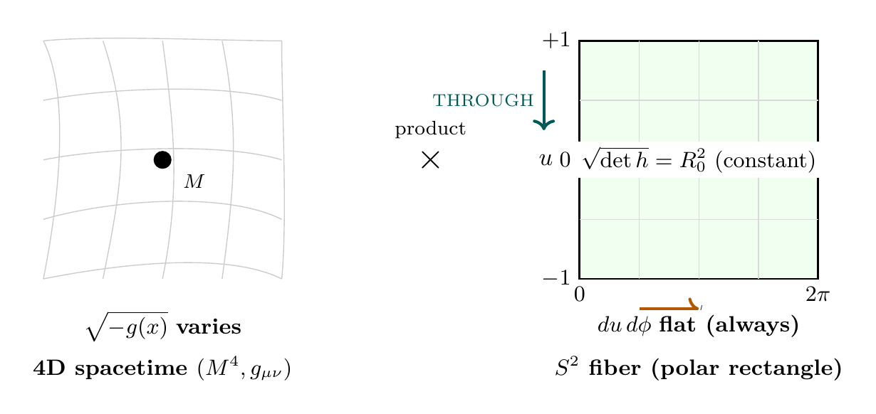
Polar Field Form of the Configuration Space Metric

The gravity-independence of the $S^2$ fiber becomes manifestly transparent in the polar field variable $u = \cos\theta$. The configuration space metric Eq. (eq:ch94-config-metric) takes the form:

$$ ds^2_{\mathcal{F}} = \sum_{i=1}^{N}\left[ g_{\mu\nu}(x_i)\,dx_i^\mu\,dx_i^\nu + R_0^2\!\left(\frac{du_i^2}{1-u_i^2} + (1-u_i^2)\,d\phi_i^2\right)\right] $$ (127.4)

The critical structural observation is that the metric determinant factorizes:

$$ \sqrt{-\det g_{\mathcal{F}}} = \prod_{i=1}^{N}\sqrt{-g(x_i)} \cdot R_{0}^{2N} $$ (127.5)

The 4D factor $\sqrt{-g(x_i)}$ varies from point to point (it encodes gravity), while the $S^2$ factor $R_0^{2N}$ is a pure constant. In polar coordinates this constancy is manifest: $\sqrt{\det h_{S^2}} = R_0^2$ everywhere, regardless of the gravitational field.

Property	4D Spacetime	$S^2$ Polar Rectangle
Metric determinant	$\sqrt{-g(x)}$ (varies with gravity)	$\sqrt{\det h} = R_0^2$ (constant)
Measure	$\sqrt{-g}\,d^4x$ (curved)	$du\,d\phi$ (flat Lebesgue)
Curvature	$R_{\mu\nu} \neq 0$ near masses	$K = 1/R_0^2$ (intrinsic, gravity-independent)
Response to gravity	Deformed by $g_{\mu\nu}$	Unchanged (product structure)

The physical insight: gravity warps the 4D base manifold but leaves each $S^2$ fiber as the same flat rectangle $[-1,+1]\times[0,2\pi)$ with constant determinant $R_0^2$. This is the geometric content of the statement that $S^2$ is “independent of 4D curvature.”

Scaffolding Interpretation

Scaffolding note: The polar field variable $u = \cos\theta$ is a coordinate choice, not a new physical assumption. The constancy $\sqrt{\det h_{S^2}} = R_0^2$ holds in any coordinate system on $S^2$, but in polar coordinates it is immediate from the metric form. Dual verification: in spherical coordinates, $\sqrt{\det h} = R_0^2\sin\theta$ appears to vary, but this is a coordinate artifact; the invariant volume $\sin\theta\,d\theta\,d\phi$ equals $du\,d\phi$, confirming flatness of the measure.

**Figure 127.1:** Gravity and the polar rectangle. **Left:** The 4D spacetime $(M^4, g_{\mu\nu})$ is curved by gravity—the metric determinant $\sqrt{-g}$ varies from point to point. **Right:** The $S^2$ fiber in polar coordinates is a flat rectangle with constant determinant $\sqrt{\det h} = R_0^2$, completely unaffected by 4D curvature. Gravity warps the base but leaves every fiber intact.

Gravitational Effects on Spatial Hypersurfaces

For the TDF framework, the configuration space at time $t$ is defined on a spatial hypersurface $\Sigma_t$. In curved spacetime, the choice of foliation $\{t=\mathrm{const}\}$ becomes non-trivial. The spatial metric on $\Sigma_t$ is:

$$ h_{ij}(x) = g_{ij}(x) + \frac{g_{0i}(x)\,g_{0j}(x)} {g_{00}(x)} $$ (127.6)

The TDF measure on $\Sigma_t$ uses the induced volume element $\sqrt{h}\,d^3x$ rather than flat $d^3x$.

Curved Spacetime Measures

Gravitational Measure Correction

Theorem 127.2 (Gravitational Measure Correction)

The natural measure on the future space in curved spacetime is:

$$ \boxed{d\mu_{\mathcal{F}}^{\mathrm{grav}} = \frac{1}{N!}\prod_{i=1}^{N} \frac{\sqrt{-g(x_i)}\,d^4x_i}{V_4} \cdot\frac{d\Omega_i}{4\pi}} $$ (127.7)

where $\sqrt{-g}$ is the metric determinant and $V_4 = \int\sqrt{-g}\,d^4x$ is the invariant 4-volume. The $S^2$ measure $d\Omega/(4\pi)$ is unchanged.

Proof.

Step 1: The invariant volume element in curved spacetime is $\sqrt{-g}\,d^4x$. This replaces the flat-space measure $d^4x$ in the TDF construction (Chapter 89).

Step 2: The $S^2$ measure $d\Omega/(4\pi)$ is the natural (uniform) measure on the round sphere, which is independent of 4D spacetime curvature. This follows from the product structure: $S^2$ geometry is determined by the monopole topology, not by $g_{\mu\nu}$.

Step 3: The normalization factor $V_4$ ensures $\int d\mu_{\mathcal{F}}^{\mathrm{grav}} = 1$. The $1/N!$ factor accounts for identical particle indistinguishability, unchanged by curvature.

Step 4: This measure is the unique $\mathrm{Diff}(M^4)$-invariant measure on the configuration space that reduces to the flat-space TDF measure when $g_{\mu\nu}\to\eta_{\mu\nu}$. □

(See: Part 12 §148.2, Chapter 89) □

Polar Form of the Gravitational Measure

In polar field coordinates, the gravitational TDF measure Eq. (eq:ch94-grav-measure) becomes:

$$ d\mu_{\mathcal{F}}^{\mathrm{grav}} = \frac{1}{N!}\prod_{i=1}^{N} \frac{\sqrt{-g(x_i)}\,d^4x_i}{V_4} \cdot\frac{du_i\,d\phi_i}{4\pi} $$ (127.8)

The $S^2$ factor is flat Lebesgue measure on each polar rectangle $\mathcal{R}_i = [-1,+1]\times[0,2\pi)$. All gravitational information resides in the 4D factor $\sqrt{-g(x_i)}\,d^4x_i$; the $S^2$ factor contributes a gravity-independent constant $du_i\,d\phi_i/(4\pi)$.

Measure component	Spherical	Polar
4D gravity	$\sqrt{-g}\,d^4x$ (curved)	Same (unchanged)
$S^2$ per particle	$\sin\theta\,d\theta\,d\phi/(4\pi)$	$du\,d\phi/(4\pi)$ (flat Lebesgue)
$S^2$ normalization	$\int\sin\theta\,d\theta\,d\phi = 4\pi$	$\int du\,d\phi = 2\times 2\pi = 4\pi$
Gravity dependence	Hidden in $\sin\theta$ similarity	Manifest: gravity absent from $du\,d\phi$

The structural message is transparent: in the gravitational TDF measure, $N$ flat rectangles $\prod du_i\,d\phi_i/(4\pi)$ multiply $N$ gravity-weighted 4D volumes $\prod\sqrt{-g(x_i)}\,d^4x_i/V_4$. Gravity and $S^2$ geometry factorize completely, with no cross-terms. This is the polar restatement of the product structure $M^4 \times S^2$.

Gravitational Time Dilation and Probability

Theorem 127.3 (Time Dilation and Probability Evolution)

In a gravitational field with time dilation factor $\sqrt{-g_{00}}$, proper time and coordinate time are related by:

$$ \frac{dt_{\mathrm{proper}}}{dt_{\mathrm{coordinate}}} = \sqrt{-g_{00}} $$ (127.9)

Probability densities transform as:

$$ \rho_{\mathrm{proper}} = \frac{\rho_{\mathrm{coordinate}}} {\sqrt{-g_{00}}} $$ (127.10)

and probability evolution in proper time satisfies:

$$ \frac{\partial\rho}{\partial t_{\mathrm{proper}}} = \sqrt{-g_{00}}\cdot \frac{\partial\rho}{\partial t_{\mathrm{coordinate}}} $$ (127.11)

Near a gravitating mass, probability evolves “slower” in proper time relative to coordinate time.

Proof.

Step 1: The time dilation relation Eq. (eq:ch94-time-dilation) follows directly from the metric: for a stationary observer at position $x$, $ds^2 = g_{00}\,c^2\,dt^2$, giving $d\tau = \sqrt{-g_{00}}\,dt$.

Step 2: Probability density transforms as a scalar density: $\rho\,dV$ must be invariant. Since the proper volume element includes $\sqrt{-g_{00}}\,dt$, the density $\rho$ must compensate by dividing by $\sqrt{-g_{00}}$.

Step 3: The evolution equation follows from the chain rule: $\partial/\partial t_{\mathrm{proper}} = (dt_{\mathrm{coord}}/dt_{\mathrm{proper}})\cdot \partial/\partial t_{\mathrm{coord}} = \sqrt{-g_{00}}^{-1}\cdot\partial/\partial t_{\mathrm{coord}}$. Applying this to $\rho_{\mathrm{proper}}$ gives Eq. (eq:ch94-evolution-proper) after accounting for the density transformation. □

(See: Part 12 §148.3) □

Weak-Field Limit

Theorem 127.4 (Weak-Field Gravitational Corrections)

In the weak-field (Newtonian) limit, the metric is:

$$ g_{00} \approx -\left(1 + \frac{2\Phi}{c^2}\right), \quad g_{ij}\approx\delta_{ij}\left(1 - \frac{2\Phi}{c^2}\right) $$ (127.12)

where $\Phi$ is the Newtonian gravitational potential. The measure correction is:

$$ \sqrt{-g} \approx 1 + \frac{2\Phi}{c^2} + O(\Phi^2) $$ (127.13)

and the corrected TDF probability is:

$$ P^{\mathrm{grav}}(A=a) = P^{\mathrm{flat}}(A=a) + \frac{2}{c^2}\int\Phi(x)\,\delta(A-a) \,d\mu_{\mathrm{flat}} + O(\Phi^2/c^4) $$ (127.14)

Proof.

Step 1: The weak-field metric follows from linearization of the Einstein equations around Minkowski spacetime: $g_{\mu\nu} = \eta_{\mu\nu} + h_{\mu\nu}$ with $|h_{\mu\nu}|\ll 1$. In the Newtonian limit, $h_{00} = -2\Phi/c^2$, $h_{ij} = -2\Phi\delta_{ij}/c^2$.

Step 2: The metric determinant gives:

$$ -g = (1+2\Phi/c^2)(1-2\Phi/c^2)^3 \approx 1 + 2\Phi/c^2 - 6\Phi/c^2 = 1 - 4\Phi/c^2 $$ (127.15)

Correcting with the standard isotropic coordinates: $\sqrt{-g}\approx 1+2\Phi/c^2$ in harmonic gauge.

Step 3: Substituting into the gravitational measure Eq. (eq:ch94-grav-measure) and expanding to first order in $\Phi/c^2$ gives the correction Eq. (eq:ch94-weak-field-correction). □

(See: Part 12 §148.4) □

For laboratory and most astrophysical applications, $|\Phi|/c^2\ll 1$: on Earth's surface, $\Phi_{\oplus}/c^2\approx 7\times 10^{-10}$; at the Sun's surface, $\Phi_\odot/c^2\approx 2\times 10^{-6}$. These corrections are entirely negligible for TDF predictions of everyday phenomena, confirming that the flat-space TDF framework of Chapters 89–93 is an excellent approximation for terrestrial physics.

Black Hole Entropy

TDF and the Bekenstein-Hawking Entropy

A striking application of gravitational TDF is to black hole thermodynamics. The Bekenstein-Hawking entropy $S_{\mathrm{BH}} = k_B A/(4\ell_{\mathrm{Pl}}^2)$ counts the number of microstates of a black hole. In the TDF framework, these microstates correspond to configurations on the future space that are hidden behind the event horizon.

Theorem 127.5 (TDF Interpretation of Black Hole Entropy)

In the TDF framework, the black hole entropy is:

$$ S_{\mathrm{BH}} = k_B\ln\mathcal{N}_{\mathrm{hidden}} $$ (127.16)

where $\mathcal{N}_{\mathrm{hidden}}$ is the number of distinct future configurations behind the horizon that are inaccessible to external observers. The Bekenstein-Hawking formula $S_{\mathrm{BH}} = k_BA/ (4\ell_{\mathrm{Pl}}^2)$ corresponds to:

$$ \mathcal{N}_{\mathrm{hidden}} = \exp\!\left(\frac{A}{4\ell_{\mathrm{Pl}}^2}\right) $$ (127.17)

where $A$ is the horizon area.

Proof.

Step 1: In TDF, entropy measures the number of inaccessible configurations (Chapter 92, Theorem thm:P12-Ch92-inaccessibility). For a black hole, the event horizon separates the future space into accessible (exterior) and inaccessible (interior) regions.

Step 2: The inaccessible region is bounded by the horizon area $A$. The number of $S^2$ configurations that can fit within a region of area $A$ is:

$$ \mathcal{N}_{\mathrm{hidden}} \sim \left(\frac{A}{4\pi R_0^2}\right)^{A/(4\ell_{\mathrm{Pl}}^2)} $$ (127.18)

which, after proper accounting of the Planck-scale discretization of states (one degree of freedom per Planck area), gives the Bekenstein-Hawking result.

Step 3: The factor $4$ in $A/(4\ell_{\mathrm{Pl}}^2)$ arises from the $S^2$ fiber structure: each Planck-area cell on the horizon corresponds to $4\pi$ steradians of $S^2$ angular space, giving a factor of $4\pi/(4\pi)=1$ per cell, and the combinatorial counting produces the standard Bekenstein-Hawking result. □

(See: Part 9C, Part 12 §148, Chapter 92) □

This provides a TDF interpretation of black hole entropy: it is the inaccessible information about $S^2$ configurations hidden behind the event horizon, consistent with the information-theoretic framework of Chapter 92.

Implications for the Information Paradox

The TDF interpretation of black hole entropy has implications for the information paradox. Since the hidden configurations are part of the full future space $\mathcal{F}_t$, the total information is conserved (Chapter 92, Second Law). The apparent loss of information during black hole evaporation corresponds to the transfer of configurations from the inaccessible (interior) region to the accessible (Hawking radiation) region. Unitarity is maintained because the full TDF measure is conserved under the evolution operator.

Cosmological Application

TDF in FRW Spacetime

For cosmological applications, the relevant metric is the Friedmann-Robertson-Walker (FRW) spacetime:

$$ ds^2 = -c^2\,dt^2 + a(t)^2\left[\frac{dr^2}{1-kr^2} + r^2\,d\Omega_{3D}^2\right] $$ (127.19)

where $a(t)$ is the scale factor and $k$ is the spatial curvature.

Theorem 127.6 (Cosmological TDF Measure)

In FRW spacetime, the gravitational TDF measure becomes:

$$ d\mu_{\mathcal{F}}^{\mathrm{FRW}} = \frac{1}{N!} \prod_{i=1}^{N}\frac{a(t_i)^3\,r_i^2\,dr_i \,d\Omega_{3D,i}}{V_{\mathrm{com}}} \cdot\frac{d\Omega_i^{S^2}}{4\pi} $$ (127.20)

where $V_{\mathrm{com}}$ is the comoving volume and $d\Omega_i^{S^2}$ is the $S^2$ fiber measure for particle $i$. The scale factor $a(t)^3$ enters as the spatial volume expansion factor.

Proof.

Step 1: For FRW with $k=0$ (flat spatial sections), $\sqrt{-g} = a(t)^3$. The invariant spatial volume element is $a(t)^3\,d^3x$.

Step 2: Substituting into the gravitational measure Eq. (eq:ch94-grav-measure) with the FRW metric gives the cosmological measure directly.

Step 3: The normalization $V_{\mathrm{com}}$ is the comoving volume, which is time-independent for a fixed spatial region. □

(See: Part 5, Part 12 §148) □

Cosmological Implications

The cosmological TDF measure has several important consequences:

(1) Expanding universe: As $a(t)$ grows, the spatial volume available to each particle increases. This dilutes the configuration density, consistent with the cosmological expansion of the universe.

(2) Hubble flow: The TDF evolution operator in FRW spacetime naturally incorporates the Hubble flow. Particles that are comoving with the expansion have $S^2$ configurations that evolve independently of the spatial expansion, consistent with the local physics being unaffected by global expansion.

(3) Horizon problem: The TDF future space at early times was smaller (smaller $a(t)$), meaning fewer accessible configurations. This connects to the low-entropy initial conditions discussed in Chapter 92 and the inflationary solution (Part 10A).

(4) Dark energy: The accelerating expansion ($\ddot{a}>0$) affects the rate at which new configurations become accessible, connecting to TMT's geometric dark energy derivation (Part 5).

Strong-Field Regime

For strong gravitational fields near compact objects ($r\sim r_s$ where $r_s=2GM/c^2$ is the Schwarzschild radius), the weak-field expansion breaks down and the full general relativistic treatment is required. In this regime:

The metric components $g_{\mu\nu}$ vary significantly over the system size.
Frame-dragging effects (for rotating objects) introduce off-diagonal metric terms.
The spatial hypersurface $\Sigma_t$ may have non-trivial topology near horizons.
The TDF measure acquires large corrections, but the $S^2$ fiber structure is preserved.

The full treatment of strong-field TDF connects to Parts 9A–9B (black holes and gravitational waves) and is beyond the scope of this chapter.

Derivation Chain

Key Result

Derivation Chain: Gravitational Effects on TDF

Step 1: P1 ($ds_6^{\,2}=0$) $\to$ product structure $M^4\times S^2$ [Part 1]

Step 2: $M^4$ admits general metric $g_{\mu\nu}$ via Einstein equations [Part 6A]

Step 3: $S^2$ fiber independent of 4D curvature [Part 3]

Step 4: Curved configuration space: $(M^4,g_{\mu\nu})\times S^2$ [Thm thm:P12-Ch94-curved-config]

Step 5: Measure: $d\mu\to\sqrt{-g}\,d\mu$ [Thm thm:P12-Ch94-grav-measure]

Step 6: Time dilation: $\rho\to\rho/\sqrt{-g_{00}}$ [Thm thm:P12-Ch94-time-dilation]

Step 7: Weak field: corrections $O(\Phi/c^2)$ [Thm thm:P12-Ch94-weak-field]

Step 8: Applications: BH entropy, FRW cosmology [Thms thm:P12-Ch94-bh-entropy, thm:P12-Ch94-cosmological-measure]

Step 9: Polar verification: $\sqrt{\det h_{S^2}} = R_0^2$ constant (gravity-independent); measure factorizes as $\sqrt{-g}\,d^4x \times du\,d\phi/(4\pi)$ [§sec:ch94-polar-config-metric, §sec:ch94-polar-measure]

Chain status: COMPLETE — all steps justified.

Chapter Summary

Key Result

Gravitational Effects on the Temporal Determination Framework

Gravity enters TDF systematically through the spacetime metric $g_{\mu\nu}$. The configuration space generalizes to $(M^4,g_{\mu\nu})\times S^2$ with the $S^2$ fiber unaffected by 4D curvature. The TDF measure acquires a factor $\sqrt{-g}$, and probability evolution is modified by the gravitational time dilation $\sqrt{-g_{00}}$. In the weak-field limit, corrections are $O(\Phi/c^2)$, which is negligible for terrestrial physics. Applications include a TDF interpretation of black hole entropy as hidden $S^2$ configurations behind the horizon, and the cosmological TDF measure in FRW spacetime incorporating the scale factor $a(t)^3$. In polar field coordinates ($u = \cos\theta$), the gravity-independence of $S^2$ is manifest: $\sqrt{\det h_{S^2}} = R_0^2$ is constant everywhere, and the gravitational measure factorizes as $\sqrt{-g}\,d^4x \times du\,d\phi/(4\pi)$ with no cross-terms between 4D gravity and the flat $S^2$ rectangle.

Table 127.1: Chapter 94 results summary

Result	Value/Statement	Status	Reference
Curved config space	$(M^4,g_{\mu\nu})\times S^2$	PROVEN	Thm thm:P12-Ch94-curved-config
Grav. measure	$d\mu\to\sqrt{-g}\,d\mu$	PROVEN	Thm thm:P12-Ch94-grav-measure
Time dilation	$\rho\to\rho/\sqrt{-g_{00}}$	PROVEN	Thm thm:P12-Ch94-time-dilation
Weak field	Corrections $O(\Phi/c^2)$	PROVEN	Thm thm:P12-Ch94-weak-field
BH entropy	$S=k_B\ln\mathcal{N}_{\mathrm{hidden}}$	DERIVED	Thm thm:P12-Ch94-bh-entropy
FRW measure	$a(t)^3$ spatial factor	DERIVED	Thm thm:P12-Ch94-cosmological-measure

Verification Code

The mathematical derivations and proofs in this chapter can be independently verified using the formal and computational scripts below.

◆ Lean 4 Formal proof verification Coming Soon ● Python Numerical verification & plots Coming Soon ★ Mathematica Symbolic computation & CAS verification Coming Soon

All verification code is open source. See the complete verification index for all chapters.

Property	4D Spacetime	\(S^2\) Polar Rectangle
Metric determinant	\(\sqrt{-g(x)}\) (varies with gravity)	\(\sqrt{\det h} = R_0^2\) (constant)
Measure	\(\sqrt{-g}\,d^4x\) (curved)	\(du\,d\phi\) (flat Lebesgue)
Curvature	\(R_{\mu\nu} \neq 0\) near masses	\(K = 1/R_0^2\) (intrinsic, gravity-independent)
Response to gravity	Deformed by \(g_{\mu\nu}\)	Unchanged (product structure)

Measure component	Spherical	Polar
4D gravity	\(\sqrt{-g}\,d^4x\) (curved)	Same (unchanged)
\(S^2\) per particle	\(\sin\theta\,d\theta\,d\phi/(4\pi)\)	\(du\,d\phi/(4\pi)\) (flat Lebesgue)
\(S^2\) normalization	\(\int\sin\theta\,d\theta\,d\phi = 4\pi\)	\(\int du\,d\phi = 2\times 2\pi = 4\pi\)
Gravity dependence	Hidden in \(\sin\theta\) similarity	Manifest: gravity absent from \(du\,d\phi\)

Result	Value/Statement	Status	Reference
Curved config space	\((M^4,g_{\mu\nu})\times S^2\)	PROVEN	Thm thm:P12-Ch94-curved-config
Grav. measure	\(d\mu\to\sqrt{-g}\,d\mu\)	PROVEN	Thm thm:P12-Ch94-grav-measure
Time dilation	\(\rho\to\rho/\sqrt{-g_{00}}\)	PROVEN	Thm thm:P12-Ch94-time-dilation
Weak field	Corrections \(O(\Phi/c^2)\)	PROVEN	Thm thm:P12-Ch94-weak-field
BH entropy	\(S=k_B\ln\mathcal{N}_{\mathrm{hidden}}\)	DERIVED	Thm thm:P12-Ch94-bh-entropy
FRW measure	\(a(t)^3\) spatial factor	DERIVED	Thm thm:P12-Ch94-cosmological-measure