Geometry of the 2-Sphere
In Chapter 8, we proved that \(\mathcal{K}^2 = S^2\) is uniquely selected by five independent physical consistency conditions. In this chapter, we develop the detailed geometry of \(S^2\) that underlies all subsequent TMT calculations. This is a technical chapter, establishing the mathematical toolkit: coordinates, metric, curvature, volume, isometries, homotopy, and the embedding chain \(S^2 \subset \mathbb{R}^3 \subset \mathbb{C}^3\) that connects the projection structure to the full Standard Model gauge group.
Throughout this chapter, “\(S^2\)” refers to the projection structure — the mathematical encoding of how 4D physics appears when observed from within 3D. The geometric properties derived here (curvature, volume, isometries, etc.) are properties of the projection interface, not of a physical 2D surface embedded in hidden extra dimensions. The 6D formalism \(\mathcal{M}^4 \times S^2\) is mathematical scaffolding for computing 4D observables.
Coordinates on \(S^2\): \((\theta, \phi)\)
The standard coordinates on \(S^2\) are the polar angle \(\theta\) and azimuthal angle \(\phi\):
The 2-sphere \(S^2\) of radius \(R\) is parametrized by:
In Cartesian ambient coordinates \(\mathbb{R}^3\), a point on \(S^2\) is:
Coordinate singularities:
- At \(\theta = 0\) (north pole): \(\phi\) is undefined
- At \(\theta = \pi\) (south pole): \(\phi\) is undefined
These are coordinate singularities, not physical singularities. The sphere is smooth everywhere. For global calculations, one uses overlapping coordinate patches (north and south charts) or works with coordinate-independent quantities.
TMT conventions (used throughout the book):
| Symbol | Range | Meaning |
|---|---|---|
| \(\theta\) | \([0, \pi]\) | Polar angle from north pole |
| \(\phi\) | \([0, 2\pi)\) | Azimuthal angle |
| \(R\) | \(> 0\) | Radius (scale parameter of projection structure) |
| \(d\Omega\) | \(\sin\theta\,d\theta\,d\phi\) | Area element on unit \(S^2\) |
| \(a, b\) | \(1, 2\) | \(S^2\) coordinate indices (\(\theta, \phi\)) |
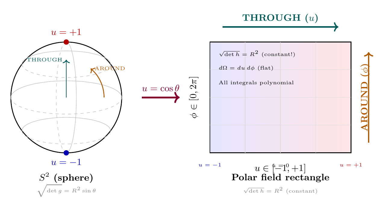
Polar Field Coordinates: \(u = \cos\theta\)
Throughout the remainder of this book, we systematically use the polar field variable:
The change \(u = \cos\theta\) is NOT a new physical assumption. It is a coordinate choice that reveals structure hidden by trigonometric expressions. In particular, the metric determinant becomes constant (\(\sqrt{\det h_{ab}} = R^2\)), all monopole harmonics become polynomial in \(u\), and the around/through decomposition becomes mathematically literal.
The key conversions from spherical to polar field coordinates are:
| Quantity | Spherical \((\theta, \phi)\) | Polar field \((u, \phi)\) |
|---|---|---|
| Variable | \(\theta \in [0, \pi]\) | \(u = \cos\theta \in [-1, +1]\) |
| Differential | \(d\theta\) | \(du / \sqrt{1-u^2}\) |
| \(\sin\theta\) | \(\sin\theta\) | \(\sqrt{1-u^2}\) |
| Area element | \(\sin\theta\,d\theta\,d\phi\) | \(du\,d\phi\) (flat!) |
| \(\sqrt{\det g}\) | \(R^2\sin\theta\) (angular) | \(R^2\) (constant) |
| North pole | \(\theta = 0\) | \(u = +1\) |
| South pole | \(\theta = \pi\) | \(u = -1\) |
| Equator | \(\theta = \pi/2\) | \(u = 0\) |
The physical interpretation: \(\phi\) parametrizes the around direction (gauge/topology), while \(u\) parametrizes the through direction (mass/dynamics). Every \(S^2\) overlap integral factorizes:
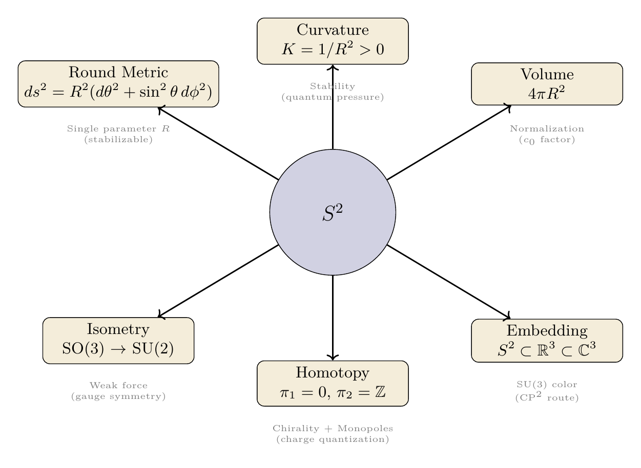
The Round Metric: \(ds^2 = R^2(d\theta^2 + \sin^2\theta\,d\phi^2)\)
In matrix form, the metric tensor \(g_{ab}\) on \(S^2\) is:
with inverse:
and determinant:
Key properties of the round metric:
- Signature: \((+, +)\) — both eigenvalues positive (Riemannian)
- Homogeneity: Every point on \(S^2\) looks the same (transitive isometry group)
- Isotropy: Every direction at any point looks the same
- Uniqueness: The round metric is the unique (up to scale) metric on \(S^2\) with these symmetries
- Single parameter: The metric is completely determined by one parameter \(R\) (no shape moduli)
The scalar Laplacian on \(S^2\) (used extensively in subsequent chapters) is:
Its eigenfunctions are the spherical harmonics \(Y_\ell^m(\theta, \phi)\):
with degeneracy \(2\ell + 1\) for each \(\ell\).
The Round Metric in Polar Field Coordinates
In the polar field variable \(u = \cos\theta\), the round metric becomes:
The metric tensor in \((u, \phi)\) coordinates is:
with constant determinant:
This is the central simplification: \(\sqrt{\det h} = R^2\) is independent of position. Every integral on \(S^2\) uses the flat measure \(du\,d\phi\) with no angular weight.
The scalar Laplacian in polar field coordinates:
Compare with eq:ch9-laplacian: the \(\sin\theta\) factors have been absorbed into the coordinate change, leaving a self-adjoint operator with respect to flat measure.
| Property | Spherical \((\theta, \phi)\) | Polar field \((u, \phi)\) |
|---|---|---|
| Metric \(ds^2\) | \(R^2(d\theta^2 + \sin^2\theta\,d\phi^2)\) | \(R^2[du^2/(1-u^2) + (1-u^2)\,d\phi^2]\) |
| \(g_{\theta\theta}\) or \(h_{uu}\) | \(R^2\) | \(R^2/(1-u^2)\) |
| \(g_{\phi\phi}\) or \(h_{\phi\phi}\) | \(R^2\sin^2\theta\) | \(R^2(1-u^2)\) |
| \(\sqrt{\det g}\) | \(R^2\sin\theta\) (varies) | \(R^2\) (constant!) |
| Area element | \(R^2\sin\theta\,d\theta\,d\phi\) | \(R^2\,du\,d\phi\) (flat) |
| Domain | \([0,\pi] \times [0, 2\pi)\) (curved) | \([-1,+1] \times [0, 2\pi)\) (rectangle) |
Curvature: \(R_{S^2} = 2/R^2\)
For the round \(S^2\) of radius \(R\):
- Gaussian curvature: \(K = 1/R^2\) (constant, positive)
- Ricci scalar: \(R_{S^2} = 2K = 2/R^2\)
- Riemann tensor: \(R_{abcd} = K(g_{ac}g_{bd} - g_{ad}g_{bc})\) (maximally symmetric)
- Ricci tensor: \(R_{ab} = Kg_{ab} = g_{ab}/R^2\)
Step 1: Compute the Christoffel symbols from the metric eq:ch9-metric-tensor. The non-vanishing components are:
Step 2: Compute the Riemann tensor \(R^\theta{}_{\phi\theta\phi}\):
Step 3: The Gaussian curvature:
Step 4: The Ricci scalar in 2D: \(R_{S^2} = 2K = 2/R^2\).
Step 5: Verify via Gauss-Bonnet:
(See: Part 2 §4.2.4) □
Physical significance of positive curvature: As shown in Chapter 8, positive curvature is one of the five properties that uniquely select \(S^2\). In the modulus stabilization mechanism, the positive curvature ensures \(c_0 > 0\) in the loop potential \(V_{\text{loop}} = c_0/R^4\), providing the quantum pressure that prevents collapse.
Volume: \(\mathrm{Vol}(S^2) = 4\pi R^2\)
Step 1: The area element on \(S^2\) with metric eq:ch9-metric-tensor:
Step 2: Integrate over the full sphere:
For the unit sphere (\(R = 1\)), \(\mathrm{Vol}(S^2) = 4\pi\). This factor appears throughout TMT calculations:
- The \(1/(4\pi)\) normalization in the loop coefficient \(c_0 = 1/(256\pi^3)\) arises from \(1/\mathrm{Vol}(S^2_{\text{unit}})\)
- Spherical harmonic orthogonality: \(\int_{S^2} Y_\ell^m (Y_{\ell'}^{m'})^*\,d\Omega = \delta_{\ell\ell'}\delta_{mm'}\)
- The participation ratio \(\int |Y_1^m|^4\,d\Omega = 1/\pi\) is normalized relative to \(\mathrm{Vol}(S^2_{\text{unit}}) = 4\pi\)
Polar field verification: In polar coordinates, the same calculation is immediate:
Isometry Group: \(\mathrm{Iso}(S^2) = \mathrm{SO}(3)\)
The isometry group of the round \(S^2\) is:
- \(\dim(\mathrm{SO}(3)) = 3\)
- Lie algebra: \(\mathfrak{so}(3) \cong \mathfrak{su}(2)\)
- Local isomorphism: \(\mathrm{SU}(2) \to \mathrm{SO}(3)\) (double cover)
Step 1: An isometry of \(S^2 \subset \mathbb{R}^3\) must preserve the metric \(ds_{S^2}^2\), which is inherited from the ambient \(\mathbb{R}^3\) metric. Any isometry of \(S^2\) extends to an orthogonal transformation of \(\mathbb{R}^3\) that maps the sphere to itself.
Step 2: The group of orthogonal transformations preserving the sphere \(\{x^2 + y^2 + z^2 = R^2\}\) is exactly O(3).
Step 3: O(3) = SO(3) \(\times\) \(\{I, -I\}\). The orientation-preserving subgroup is SO(3), with \(\dim = 3\).
Step 4: The Lie algebra \(\mathfrak{so}(3)\) consists of \(3 \times 3\) antisymmetric matrices, spanned by:
(See: Part 2 §4.5.1, App 2A) □
Killing vectors on \(S^2\): The three generators of SO(3) correspond to the Killing vector fields on \(S^2\):
These satisfy \([\xi_a, \xi_b] = \epsilon_{abc}\xi_c\) and generate the SO(3) \(\cong\) SU(2) gauge symmetry in TMT. The average squared norm:
Physical significance: In Kaluza-Klein reduction on \(S^2\), these isometries generate the SU(2) gauge fields of the weak interaction. The Killing vectors become the gauge potentials \(A_\mu^a\) after dimensional reduction.
Polar field form of Killing vectors: In \((u, \phi)\) coordinates (cf. §sec:ch8-polar-isometry):
Homotopy: \(\pi_1 = 0\), \(\pi_2 = \mathbb{Z}\)
The low-dimensional homotopy groups of \(S^2\) are:
Physical consequences of each:
\(\pi_1(S^2) = 0\) (simply connected):
- Every loop on \(S^2\) can be contracted to a point
- Consequence: unique spin structure (shown in Ch. 8), enabling chirality
- Consequence: no topological defects of the “cosmic string” type
- The fundamental group being trivial means \(H^1(S^2; \mathbb{Z}_2) = 0\), giving \(N_{\mathrm{spin}} = 2^0 = 1\)
\(\pi_2(S^2) = \mathbb{Z}\) (non-trivial second homotopy):
- Maps \(S^2 \to S^2\) are classified by integer winding number \(n \in \mathbb{Z}\)
- Consequence: magnetic monopoles exist on \(S^2\), with monopole charge \(n\)
- U(1) bundles over \(S^2\) are classified by the first Chern class \(c_1 \in H^2(S^2; \mathbb{Z}) \cong \pi_2(S^2) \cong \mathbb{Z}\)
- Dirac quantization: the monopole charge \(n\) determines the allowed matter charges through \(qn \in \mathbb{Z}\)
- Energy minimization: \(E \propto n^2\) selects \(|n| = 1\) as the ground state
Summary of homotopy consequences:
| Group | Value | Physical Consequence |
|---|---|---|
| \(\pi_0\) | \(0\) | \(S^2\) is connected (single projection structure) |
| \(\pi_1\) | \(0\) | Simply connected \(\to\) unique spin structure \(\to\) chirality |
| \(\pi_2\) | \(\mathbb{Z}\) | Monopoles \(\to\) charge quantization \(\to\) Higgs structure |
The Embedding Chain
The embedding chain \(S^2 \subset \mathbb{R}^3 \subset \mathbb{C}^3\) describes mathematical relationships between structures, not physical containment of spaces within spaces. “\(S^2\) embeds in \(\mathbb{R}^3\)” means the projection structure has mathematical properties requiring 3 real dimensions to describe without pathologies. “\(\mathbb{R}^3 \subset \mathbb{C}^3\)” means quantum mechanics requires complexification of the ambient space.
\(S^2 \subset \mathbb{R}^3\) (Minimal Embedding)
\(S^2\) embeds in \(\mathbb{R}^3\) as \(\{(x, y, z) \in \mathbb{R}^3 : x^2 + y^2 + z^2 = R^2\}\). This embedding is:
- Smooth: The map is \(C^\infty\)
- Isometric: It preserves the round metric
- Minimal: \(S^2\) cannot embed in \(\mathbb{R}^2\) (it would self-intersect)
Therefore \(\mathbb{R}^3\) is the minimal ambient Euclidean space for \(S^2\).
Step 1 (Lower bound): \(S^2\) is a compact, orientable 2-manifold. By the Jordan-Brouwer separation theorem (Brouwer 1912), \(S^2\) separates \(\mathbb{R}^3\) into “inside” and “outside” regions. In \(\mathbb{R}^2\), a closed 2-manifold cannot embed without self-intersection. Therefore \(\dim \geq 3\).
Step 2 (Achievability): The standard embedding \(x^2 + y^2 + z^2 = R^2\) realizes \(S^2\) in \(\mathbb{R}^3\).
Step 3 (Minimality): Since \(\dim \geq 3\) is required and \(\dim = 3\) is achieved, \(\mathbb{R}^3\) is minimal.
Note: The Whitney embedding theorem guarantees any smooth compact \(n\)-manifold embeds in \(\mathbb{R}^{2n}\), giving \(S^2 \subset \mathbb{R}^4\). The standard embedding achieves better: \(S^2 \subset \mathbb{R}^3\). □
(See: Part 2 §5.1) □
This embedding is forced by topology, not chosen. The mathematical properties of \(S^2\) require at least 3 real dimensions for an embedding without self-intersection.
\(\mathbb{R}^3 \subset \mathbb{C}^3\) (QM Complexification)
Quantum mechanical state spaces are complex Hilbert spaces.
Step 1: Superposition: \(|\psi\rangle = \alpha|0\rangle + \beta|1\rangle\) with \(\alpha, \beta\) complex.
Step 2: Normalization: \(|\alpha|^2 + |\beta|^2 = 1\).
Step 3: The phase \(\alpha = |\alpha|e^{i\phi}\) is physically observable (via interference).
Step 4: A real Hilbert space has no phase structure \(\to\) no interference patterns.
Step 5: Interference is experimentally observed \(\to\) complex Hilbert space required. □
(See: Part 2 §5.2) □
The complexification of \(\mathbb{R}^3\) is:
“Fields take values in \(\mathbb{C}^3\)” does NOT mean fields are “living on” a literal 6D space \(\mathcal{M}^4 \times S^2\). Rather, 4D quantum fields, when their coupling to the \(S^2\) projection structure is made explicit, naturally have components that transform under the \(\mathbb{C}^3\) structure. \(\mathbb{C}^3\) is the natural internal space for these interactions, not an additional physical dimension.
Quantum fields on \(\mathcal{M}^4 \times S^2\) with ambient-space indices take values in \(\mathbb{C}^3\).
Step 1: \(S^2 \hookrightarrow \mathbb{R}^3\) (minimal embedding, Theorem thm:P2-Ch9-minimal-embedding).
Step 2: Fields have indices from the ambient space \(\mathbb{R}^3\).
Step 3: QM requires complex field values (Theorem thm:P2-Ch9-qm-complex).
Step 4: Therefore field space \(= \mathbb{R}^3 \otimes \mathbb{C} = \mathbb{C}^3\). □
(See: Part 2 §5.2) □
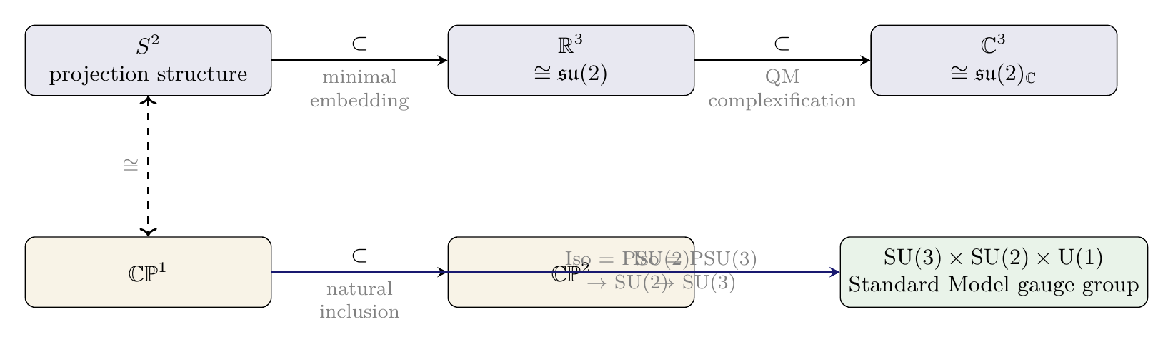
The Complete Chain: \(S^2 \subset \mathbb{R}^3 \subset \mathbb{C}^3\)
- \(S^2 \hookrightarrow \mathbb{R}^3\): minimal embedding (Whitney + Jordan-Brouwer)
- \(\mathbb{R}^3 \hookrightarrow \mathbb{C}^3\): quantum mechanics (complex Hilbert spaces)
| Step | From | To | Reason |
|---|---|---|---|
| 1 | \(S^2\) | \(\mathbb{R}^3\) | Minimal embedding (topology) |
| 2 | \(\mathbb{R}^3\) | \(\mathbb{C}^3\) | Quantum mechanics (complex structure) |
The Complex Projective Interpretation
\(S^2 \cong \mathbb{CP}^1\)
The 2-sphere is diffeomorphic to the complex projective line:
The diffeomorphism is given by stereographic projection:
This identification is profound: \(S^2\) is simultaneously a real 2-manifold and a complex 1-manifold (\(\mathbb{CP}^1\)). This dual nature connects real geometry (curvature, isometries) with complex algebraic geometry (line bundles, Chern classes).
\(\mathbb{CP}^1 \subset \mathbb{CP}^2\)
This inclusion is natural in the sense that it is the simplest way to embed \(\mathbb{CP}^1\) into the next complex projective space. It corresponds to restricting the homogeneous coordinates to a hyperplane in \(\mathbb{CP}^2\).
\(\mathrm{Iso}(\mathbb{CP}^1) = \mathrm{PSU}(2)\), \(\mathrm{Iso}(\mathbb{CP}^2) = \mathrm{PSU}(3)\)
With the Fubini-Study metric:
Key Insight: The \(S^2 = \mathbb{CP}^1\) that we observe is a subspace of \(\mathbb{CP}^2\). The SU(2) isometry is the restriction of SU(3) to this subspace.
The SU(3) was always there — we see the SU(2) part on the interface.
This is how the Standard Model gauge group emerges:
- \(\mathrm{Iso}(S^2) = \mathrm{SO}(3) \cong \mathrm{PSU}(2) = \mathrm{Iso}(\mathbb{CP}^1)\) gives the SU(2) weak interaction
- The ambient \(\mathbb{CP}^2\) has \(\mathrm{Iso}(\mathbb{CP}^2) = \mathrm{PSU}(3)\), giving the SU(3) color interaction
- The U(1) hypercharge comes from the monopole bundle on \(S^2\)
Together: \(\mathrm{SU}(3) \times \mathrm{SU}(2) \times \mathrm{U}(1)\) — the full Standard Model gauge group.
The Dimension Coincidence Explained
\(\mathfrak{su}(2) \cong \mathfrak{so}(3) \cong \mathbb{R}^3\)
An apparent coincidence pervades the structure: the embedding space \(\mathbb{R}^3\), the Lie algebra \(\mathfrak{su}(2)\), and the isometry algebra \(\mathfrak{so}(3)\) all have dimension 3. Is this numerology?
Step 1: \(\mathfrak{su}(2) = \text{traceless skew-Hermitian } 2 \times 2 \text{ matrices}\) has basis \(\{i\sigma_1, i\sigma_2, i\sigma_3\}\) where \(\sigma_i\) are the Pauli matrices. Thus \(\dim_{\mathbb{R}} = 3\).
Step 2: The isomorphism to \(\mathbb{R}^3\) is: \(i\sigma_i \mapsto e_i\) (standard basis vector).
Step 3: The isomorphism to \(\mathfrak{so}(3)\) maps \(i\sigma_a/2 \mapsto L_a\) where \(L_a\) are the SO(3) generators.
Step 4: All three carry the same Lie bracket: \([T_a, T_b] = \epsilon_{abc}T_c\) (with appropriate normalization). □
(See: Part 2 §5.5.2) □
\(\mathbb{C}^3 \cong \mathfrak{su}(2)_{\mathbb{C}}\) (Deep Unity)
The ambient space \(\mathbb{C}^3\) IS the complexified Lie algebra of SU(2)!
Physical meaning:
- The “position space” \(S^2\) has isometry generated by \(\mathfrak{su}(2) \cong \mathbb{R}^3\)
- The “field space” is \(\mathbb{C}^3 = \) complexification of \(\mathbb{R}^3\)
- Position space and field space dimensions match because they arise from the same structure
The chain of identifications:
connects the topology of the projection structure (left) to the gauge algebra of the theory (middle) to the quantum field space (right). Everything is unified through \(S^2\) geometry.
| Result | Statement | Status |
|---|---|---|
| Minimal embedding | \(S^2 \hookrightarrow \mathbb{R}^3\) | ESTABLISHED (topology) |
| Complexification | \(\mathbb{R}^3 \to \mathbb{C}^3\) | ESTABLISHED (QM) |
| Lie algebra isomorphism | \(\mathfrak{su}(2) \cong \mathfrak{so}(3) \cong \mathbb{R}^3\) | ESTABLISHED (Lie theory) |
| Deep unity | \(\mathbb{C}^3 \cong \mathfrak{su}(2)_\mathbb{C}\) | ESTABLISHED (Lie theory) |
| CP interpretation | \(S^2 \cong \mathbb{CP}^1 \subset \mathbb{CP}^2\) | ESTABLISHED (algebraic geometry) |
| Dimension coincidence | Explained, not numerology | DERIVED |
Chapter Summary
Topic: Detailed geometry of \(S^2\) — the mathematical toolkit for all subsequent TMT calculations.
Key Results:
- Metric: \(ds_{S^2}^2 = R^2(d\theta^2 + \sin^2\theta\,d\phi^2)\) — unique round metric
- Curvature: \(R_{S^2} = 2/R^2\) — constant positive curvature
- Volume: \(\mathrm{Vol}(S^2) = 4\pi R^2\)
- Isometry: \(\mathrm{Iso}(S^2) = \mathrm{SO}(3)\), \(\dim = 3\) \(\to\) SU(2) gauge
- Homotopy: \(\pi_1 = 0\) (chirality), \(\pi_2 = \mathbb{Z}\) (monopoles)
- Embedding: \(S^2 \subset \mathbb{R}^3 \subset \mathbb{C}^3\) (forced)
- CP structure: \(S^2 \cong \mathbb{CP}^1 \subset \mathbb{CP}^2\) \(\to\) SU(3) color
- Deep unity: \(\mathbb{C}^3 \cong \mathfrak{su}(2)_\mathbb{C}\) (not coincidence)
Polar field coordinates: The substitution \(u = \cos\theta\) maps \(S^2\) to the flat rectangle \([-1,+1] \times [0,2\pi)\) with constant metric determinant \(\sqrt{\det h} = R^2\). All subsequent \(S^2\) integrals become polynomial integrals in \(u\) with flat measure, and the AROUND (\(\phi\)) / THROUGH (\(u\)) decomposition is mathematically literal.
Status: All results [Status: ESTABLISHED] or [DERIVED].
What comes next: Chapter 10 introduces the Dirac monopole on \(S^2\) — why the non-trivial topology (\(\pi_2(S^2) = \mathbb{Z}\)) forces a monopole gauge field, the Dirac quantization condition \(qn \in \mathbb{Z}\), and how monopole charge quantization connects to the Standard Model hypercharge structure.
Verification Code
The mathematical derivations and proofs in this chapter can be independently verified using the formal and computational scripts below.
All verification code is open source. See the complete verification index for all chapters.