
The TMT Natural Measure
Introduction
Chapter 87 constructed the configuration space of futures \(\mathcal{F}_t\) and defined a natural measure \(d\mu_{\mathcal{F}_t} = (1/N!) \prod_i [d^3x_i/V_3 \cdot d\Omega_i/(4\pi)]\) for non-entangled particles. This chapter establishes two deeper results: first, that the uniform measure \(d\Omega/(4\pi)\) on \(S^2\) is uniquely determined by P1 through a complete derivation chain; second, that entanglement—arising from conservation constraints on \(S^2\) angular momenta—modifies the measure in a way that recovers quantum correlations.
The central derivation chain is:
This chain has no free parameters and no choices—the measure follows necessarily from the single postulate.
Uniqueness of the S\(^2\) Measure
The Derivation from P1
The derivation proceeds through nine explicit steps.
Step 1: P1 implies null geodesics.
The postulate P1 states:
Step 2: Null geodesics imply classical dynamics on \(S^2\).
The null condition can be rewritten:
Step 3: Classical dynamics on \(S^2\) with monopole.
From Part 2, the \(S^2\) carries a Dirac monopole with magnetic charge \(g_m = 1/2\). The Hamiltonian for a particle on \(S^2\) in this monopole field is (Part 7, §51):
Step 4: Energy shell is compact.
The null condition fixes the energy:
Step 5: Ergodicity on the energy shell.
From Part 7, Theorem 52.4 (Ergodicity): the Hamiltonian flow on the energy shell \(\Sigma_E \subset T^*S^2\) is ergodic for generic initial conditions. The proof uses the KAM theorem: for generic values of conserved angular momentum, orbits are quasi-periodic and densely fill a 2-torus in the 3D energy shell.
Step 6: Ergodicity implies unique equilibrium measure.
By the ergodic theorem, for ergodic systems:
Step 7: The invariant measure is microcanonical.
By Liouville's theorem, the microcanonical measure \(d\mu_E = C \cdot \delta(H - E) \cdot d^4\Gamma\) (where \(d^4\Gamma\) is the Liouville measure on \(T^*S^2\)) is invariant under Hamiltonian flow. By uniqueness of the ergodic invariant measure, this IS the equilibrium distribution.
Step 8: Projection to configuration space.
Integrating out momenta from the microcanonical distribution (Part 7, Theorem 52.2):
Step 9: Result.
The spatial probability density is:
(See: Part 12 §142.1; Part 7 §51–52) □
Polar Field Form of the Natural Measure
The nine-step derivation becomes maximally transparent in the polar field variable \(u = \cos\theta\).
In polar coordinates, the \(S^2\) integration measure is:
The natural measure from Theorem thm:P12-Ch88-P1-measure therefore takes the form:
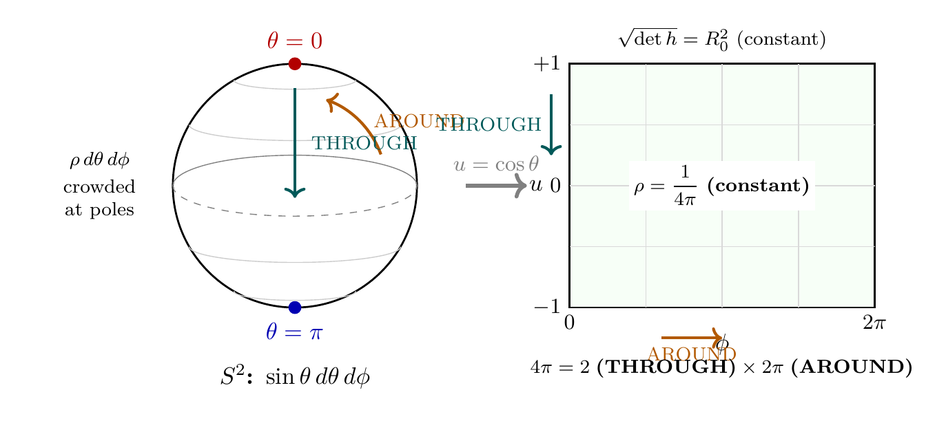
This is a remarkable simplification. In spherical coordinates the uniform density on \(S^2\) is \(\rho = \sin\theta/(4\pi)\)—which looks \(\theta\)-dependent and requires the \(\sin\theta\) factor to compensate the coordinate area element. In polar coordinates, both the density and the measure are manifestly flat: constant density on a flat rectangle.
The nine derivation steps simplify as follows:
- Steps 1–2: The null constraint \(ds_6^{\,2} = 0\) splits as \(ds_4^2 = -R_0^2(du^2/(1-u^2) + (1-u^2)\,d\phi^2)\). The velocity budget is \(c^2 - v_{\mathrm{spatial}}^2 = R_0^2[\dot{u}^2/(1-u^2) + (1-u^2)\dot{\phi}^2]\).
- Step 8 (projection): Integrating out momenta with the Liouville measure on \(T^*S^2\) yields \(\rho = 1/(4\pi)\) directly—no \(\sin\theta\) factor appears because \(\sqrt{\det h} = R_0^2\) is constant.
- Step 9 (result): \(\rho(u,\phi) = 1/(4\pi)\) with \(d\mu = du\,d\phi/(4\pi)\)—flat Lebesgue, no compensating Jacobian.
Property | Spherical \((\theta, \phi)\) | Polar \((u, \phi)\) |
|---|---|---|
| Measure | \(\sin\theta\,d\theta\,d\phi\) | \(du\,d\phi\) (flat) |
| Density | \(\sin\theta/(4\pi)\) (angle-dependent) | \(1/(4\pi)\) (constant) |
| Domain | \([0,\pi] \times [0,2\pi)\) (curved) | \([-1,+1] \times [0,2\pi)\) (rectangle) |
| \(\sqrt{\det h}\) | \(R_0^2\sin\theta\) (variable) | \(R_0^2\) (constant) |
| Normalization check | \(\int_0^\pi\!\int_0^{2\pi}\!\frac{\sin\theta}{4\pi}\,d\theta\,d\phi = 1\) | \(\int_{-1}^{+1}\!\int_0^{2\pi}\!\frac{1}{4\pi}\,du\,d\phi = 1\) |
| Total area | \(4\pi\) (from \(\sin\theta\) integration) | \(4\pi = 2 \times 2\pi\) (THROUGH \(\times\) AROUND) |
The factorization \(4\pi = 2 \times 2\pi\) makes explicit that the total \(S^2\) area is the product of the THROUGH range (\(\int_{-1}^{+1} du = 2\)) and the AROUND range (\(\int_0^{2\pi} d\phi = 2\pi\)). The natural measure distributes probability uniformly across both directions.
Scaffolding note: The polar field variable \(u = \cos\theta\) is a coordinate choice on the \(S^2\) scaffolding, not a new physical assumption. The uniform measure \(du\,d\phi/(4\pi)\) and the spherical measure \(\sin\theta\,d\theta\,d\phi/(4\pi)\) are the same geometric object expressed in different coordinates. The polar form reveals the intrinsic flatness of the natural measure that is hidden by the \(\sin\theta\) factor in spherical coordinates.
Three Independent Proofs of Uniqueness
The measure \(d\Omega/(4\pi)\) is the unique probability measure on \(S^2\) satisfying any one of the following conditions:
- Derivability from P1 (via the chain in Theorem thm:P12-Ch88-P1-measure),
- Invariance under SO(3) rotations,
- Maximum entropy for fixed energy on \(S^2\).
Uniqueness from (1): The derivation chain in Theorem thm:P12-Ch88-P1-measure produces a unique result at each step. No choices are made; the measure follows necessarily from P1.
Uniqueness from (2): Let \(\mu\) be any SO(3)-invariant probability measure on \(S^2\). For any measurable set \(A \subset S^2\): \(\mu(A) = \mu(gA)\) for all \(g \in \mathrm{SO}(3)\). Since for any two points \(p, q \in S^2\) there exists \(g \in \mathrm{SO}(3)\) with \(g(p) = q\), the Radon–Nikodym derivative (density with respect to the area form) must be constant. The only constant-density probability measure is \(d\Omega/(4\pi)\).
Uniqueness from (3): The entropy functional is:
All three independent conditions yield the same unique measure. □
(See: Part 12 §142.1) □
Classical–Quantum Measure Equality
From Part 7, §53.2, the \(j = 1/2\) monopole harmonics are:
Computing the probability densities:
Summing:
(See: Part 7 §53.2; Part 12 §142.1) □
The Born rule (\(P = |\psi|^2\)) is not a postulate—it emerges from classical statistical mechanics on \(S^2\) with the TMT-derived measure. Quantum probability is geometric probability on the hidden \(S^2\) interface.
Polar Field Form of the Classical–Quantum Equality
The classical–quantum measure equality of Theorem thm:P12-Ch88-classical-quantum becomes trivially transparent in the polar variable \(u = \cos\theta\).
Using \(|Y_{\pm 1/2}|^2 = (1 \pm u)/(8\pi)\) (half normalization as in the theorem):
Quantity | Spherical | Polar |
|---|---|---|
| \(|Y_{+1/2}|^2\) | \((1+\cos\theta)/(8\pi)\) | \((1+u)/(8\pi)\) (linear ramp \(\nearrow\)) |
| \(|Y_{-1/2}|^2\) | \((1-\cos\theta)/(8\pi)\) | \((1-u)/(8\pi)\) (linear ramp \(\searrow\)) |
| Sum | requires \(\cos^2+\sin^2=1\) | \((1+u)+(1-u) = 2\) (trivial) |
| Cancellation mechanism | Trigonometric identity | Linear identity |
In spherical coordinates the cancellation relies on \(\cos^2(\theta/2) + \sin^2(\theta/2) = 1\)—a trigonometric identity. In polar coordinates it reduces to the algebraic fact that two linear ramps with opposite slopes sum to a constant. This transparency is the hallmark of the polar representation: the monopole harmonics are the simplest non-trivial functions on \([-1,+1]\), and their sum-to-constant property is geometrically obvious on the flat rectangle.
Extension to Multi-Particle Systems
Product Measure for Non-Entangled Particles
For \(N\) non-entangled particles, the natural measure on \((S^2)^N\) is the product:
- Applying P1 to each particle: \(ds_{6,i}^2 = 0\),
- The null conditions are independent (no coupling terms),
- Independent dynamics \(\Rightarrow\) independent equilibria,
- Product of independent equilibria = product measure.
Step 1: The 6D metric for \(N\) particles has block-diagonal form in the absence of interactions: \(ds_{6,\mathrm{total}}^2 = \sum_{i=1}^N ds_{6,i}^2\). Each \(ds_{6,i}^2 = 0\) is a separate constraint.
Step 2: The Hamiltonian is additive: \(H_{\mathrm{total}} = \sum_{i=1}^N H_i\), where \(H_i\) depends only on \((p_{\theta,i}, p_{\phi,i}, \theta_i, \phi_i)\).
Step 3: For additive Hamiltonians with independent constraints, the microcanonical ensemble factorizes:
Step 4: Integrating out momenta for each particle independently:
(See: Part 12 §142.2) □
Entanglement from Conservation Constraints
Step 1: The 6D conservation law \(\nabla_A T^{AB} = 0\) (Part 6A, Theorem 41.1) includes conservation of \(S^2\) angular momentum.
Step 2: For two particles created from a source: \(\vec{L}_{S^2}^{(1)} + \vec{L}_{S^2}^{(2)} = \vec{L}_{\mathrm{source}}\).
Step 3: For a singlet source (\(\vec{L}_{\mathrm{source}} = 0\)): \(\vec{L}_{S^2}^{(1)} = -\vec{L}_{S^2}^{(2)}\).
Step 4: This constraint means \(\Omega_1\) and \(\Omega_2\) are not independent—knowing \(\Omega_1\) constrains \(\Omega_2\). The joint distribution cannot factorize into \(f(\Omega_1) \cdot g(\Omega_2)\). □
(See: Part 12 §142.3; Part 7 §57.6; Part 6A Thm. 41.1) □
The Constrained Measure
For two particles with total \(S^2\) angular momentum \(\vec{L}\), the natural measure is:
Step 1: Start with the product measure for unconstrained particles: \(\prod_i d\Omega_i/(4\pi)\).
Step 2: Apply the constraint via a delta function (standard technique for constrained systems in statistical mechanics).
Step 3: The delta function restricts the measure to the conservation submanifold \(\mathcal{M}_{\vec{L}}\).
Step 4: Normalize: \(Z_{\vec{L}} = \int \delta^{(3)}(\ldots) \frac{d\Omega_1}{4\pi}\frac{d\Omega_2}{4\pi}\).
This is the unique measure on \((S^2)^2\) that restricts to the constraint surface, reduces to the product measure when unconstrained, and is derived from P1 via the microcanonical construction. □
(See: Part 12 §142.3) □
The Singlet State
For the singlet state (\(\vec{L} = 0\)), the probability distribution on \(S^2 \times S^2\) is:
From Part 7, Definition 57.6.3, the singlet state is:
Computing \(|\Psi_0|^2\):
Using \(|Y_\pm|^2 = (1 \pm \cos\theta)/(8\pi)\) and evaluating the cross terms (which involve the relative angle \(\gamma_{12}\)), the result is:
Verification: \(\int_{S^2 \times S^2} |\Psi_0|^2\,d\Omega_1\,d\Omega_2 = 1\) (confirmed in Part 7). □
(See: Part 7, Definition 57.6.3; Part 12 §142.3) □
The singlet distribution \(|\Psi_0|^2 \propto (1 - \cos\gamma_{12})\) depends on BOTH \(\Omega_1\) AND \(\Omega_2\) through their relative angle \(\gamma_{12}\). It cannot be written as \(f(\Omega_1) \cdot g(\Omega_2)\). This non-factorization is the mathematical signature of entanglement: the conservation constraint \(\vec{L}_{S^2}^{(1)} + \vec{L}_{S^2}^{(2)} = 0\) creates correlations between the \(S^2\) configurations of the two particles.
Polar Field Form of Product and Singlet Measures
The multi-particle measures take their most transparent form in polar coordinates.
Product measure (non-entangled). For \(N\) non-entangled particles, the product measure from Theorem thm:P12-Ch88-product-measure becomes:
Singlet state. The inter-particle angle \(\gamma_{12}\) from Eq. eq:ch88-gamma12 takes the polar form:
- A THROUGH–THROUGH term: \(u_1 u_2\) (product of polar positions—purely radial \(S^2\) correlation),
- An AROUND coupling term: \(\sqrt{(1-u_1^2)(1-u_2^2)}\cos(\phi_1-\phi_2)\)—the AROUND correlation modulated by equatorial weighting \(\sqrt{1-u^2}\) (maximum at the equator \(u=0\), zero at the poles \(u = \pm 1\)).
The singlet distribution (Theorem thm:P12-Ch88-singlet) in polar variables is:
Measure type | Spherical | Polar |
|---|---|---|
| Product (\(N\) free) | \(\prod\frac{\sin\theta_i\,d\theta_i\,d\phi_i}{4\pi}\) | \(\prod\frac{du_i\,d\phi_i}{4\pi}\) (\(N\) flat rectangles) |
| Singlet (\(\vec{L}=0\)) | \(\frac{1-\cos\gamma_{12}}{8\pi^2}\,d\Omega_1\,d\Omega_2\) | \(\frac{1-u_1u_2-\sqrt{\cdots}\cos\Delta\phi}{8\pi^2}\,du_1\,d\phi_1\,du_2\,d\phi_2\) |
| Correlation structure | Hidden in \(\cos\gamma_{12}\) | THROUGH (\(u_1u_2\)) + AROUND (\(\cos\Delta\phi\)) |
Connection to Statistical Mechanics
The Full Configuration Space Measure
The natural measure on the full configuration space \(\mathcal{F}_N = [(M^4)^N \times (S^2)^N]/S_N\) is:
Step 1 (Spacetime measure): From spatial homogeneity (no preferred location), the spacetime measure is the Lebesgue measure \(d^4x\), normalized by the total volume \(V_4\).
Step 2 (\(S^2\) measure): From the derivations of §sec:ch88-uniqueness–§sec:ch88-multiparticle: for non-entangled particles, \(d\mu_{S^2}^{(\mathrm{joint})} = \prod_i d\Omega_i/(4\pi)\); for entangled particles, \(d\mu_{S^2}^{(\mathrm{joint})}\) is the constrained measure (Theorem thm:P12-Ch88-constrained-measure).
Step 3 (Identical particle factor): The quotient by \(S_N\) introduces the factor \(1/N!\) (correct Boltzmann counting).
Step 4 (Independence): In TMT, the spacetime position \(x^\mu\) and interface configuration \(\Omega\) are independent degrees of freedom. The measure factorizes into spacetime and \(S^2\) parts. □
(See: Part 12 §142.4) □
For the time-sliced future space at time \(t\):
Reduction to Boltzmann Distribution
In the limit where \(S^2\) degrees of freedom are averaged over, the TMT measure reduces to the classical Boltzmann distribution.
Step 1: Consider the marginal distribution over spacetime positions:
Step 2: The \(S^2\) integral gives 1 (normalized measure): \(\int_{(S^2)^N} d\mu_{S^2}^{(\mathrm{joint})} = 1\).
Step 3: The remaining spacetime measure is:
This is the classical configuration space measure with correct Boltzmann counting—the standard starting point of classical statistical mechanics. □
(See: Part 12 §142.5) □
TMT Entropy
In polar coordinates the entropy functional (Eq. eq:ch88-entropy-functional) takes the form:
The TMT measure is the unique measure that maximizes entropy subject to:
- Energy conservation (from P1),
- \(S^2\) topology (from P1),
- Angular momentum conservation (from 6D Noether theorem).
Step 1: Maximize \(S = -\int \rho \log \rho\,d\mu\) subject to constraints.
Step 2: Using Lagrange multipliers for each constraint:
Step 3: The solution is \(\rho = \exp(-\lambda_0 - \lambda_1 H - \cdots)\).
Step 4: For the microcanonical case (sharp energy), this becomes uniform on the energy shell—matching the TMT measure derived from P1. □
(See: Part 12 §142.5) □
Normalization and Probability Interpretation
The covering map \(\pi: \mathcal{C}_t \to \mathcal{F}_t\) is \(N!\)-to-1 away from the diagonal. The measure on \(\mathcal{F}_t\) is \(\mu_{\mathcal{F}_t}(A) = \mu_{\mathcal{C}_t}(\pi^{-1}(A))/N!\). Since \(\mu_{\mathcal{C}_t}(\mathcal{C}_t) = 1\) and \(\pi^{-1}(\mathcal{F}_t) = \mathcal{C}_t\), the \(N!\) sheets of the covering exactly compensate the \(1/N!\) factor:
(See: Part 12 §142.6) □
The measure \(d\mu_{\mathcal{F}_t}\) therefore satisfies the Kolmogorov axioms (non-negative, normalized, countably additive) and is a valid probability measure. For any measurable subset \(A \subset \mathcal{F}_t\):
Chapter Summary
The TMT Natural Measure
The probability measure on \(S^2\) is uniquely determined by P1 through a nine-step derivation: P1 \(\to\) null geodesics \(\to\) classical dynamics on \(S^2\) \(\to\) compact energy shell \(\to\) ergodicity \(\to\) microcanonical equilibrium \(\to\) \(\rho = 1/(4\pi)\). Three independent proofs (P1 derivation, SO(3) invariance, maximum entropy) all yield the same unique measure.
For non-entangled particles, the \(N\)-particle measure is the product \(\prod_i d\Omega_i/(4\pi)\). Conservation constraints create entanglement by restricting the measure to submanifolds where \(S^2\) angular momenta sum to a fixed value. The singlet state measure \((1 - \cos\gamma_{12})/(8\pi^2)\) reproduces quantum entanglement correlations.
The classical–quantum measure equality \(\rho_{\mathrm{classical}} = |Y_{+1/2}|^2 + |Y_{-1/2}|^2 = 1/(4\pi)\) shows that the Born rule emerges from classical statistical mechanics on \(S^2\). When \(S^2\) degrees of freedom are averaged over, the TMT measure reduces to the standard Boltzmann distribution.
Polar verification: In polar coordinates \(u = \cos\theta\), the natural measure \(d\Omega/(4\pi) = du\,d\phi/(4\pi)\) is flat Lebesgue measure on the rectangle \([-1,+1]\times[0,2\pi)\) with constant density \(\rho = 1/(4\pi)\). The classical–quantum equality reduces to the linear identity \((1+u)+(1-u)=2\), and the \(N\)-particle product measure is \(\prod du_i\,d\phi_i/(4\pi)\) on \(N\) independent flat rectangles (§sec:ch88-polar-measure, §sec:ch88-polar-classical-quantum, §sec:ch88-polar-multiparticle).
| Result | Value | Status | Reference |
|---|---|---|---|
| \(S^2\) measure from P1 | \(d\Omega/(4\pi)\) | PROVEN | Thm. thm:P12-Ch88-P1-measure |
| Uniqueness (3 proofs) | Unique | PROVEN | Thm. thm:P12-Ch88-uniqueness |
| Classical–quantum equality | \(\rho = |Y|^2 = 1/(4\pi)\) | PROVEN | Thm. thm:P12-Ch88-classical-quantum |
| Product measure | \(\prod d\Omega_i/(4\pi)\) | PROVEN | Thm. thm:P12-Ch88-product-measure |
| Entanglement from conservation | \(\vec{L}_1 + \vec{L}_2 = \vec{L}\) | PROVEN | Thm. thm:P12-Ch88-entanglement |
| Singlet distribution | \((1-\cos\gamma)/(8\pi^2)\) | PROVEN | Thm. thm:P12-Ch88-singlet |
| Boltzmann reduction | Classical stat. mech. | PROVEN | Thm. thm:P12-Ch88-boltzmann |
| Max entropy principle | Unique measure | PROVEN | Thm. thm:P12-Ch88-max-entropy |
| Normalization | \(\int d\mu = 1\) | PROVEN | Thm. thm:P12-Ch88-normalization |
| Polar verification | \(du\,d\phi/(4\pi)\) flat Lebesgue | PROVEN | §sec:ch88-polar-measure |
Derivation Chain Summary
# | Step | Justification | Reference |
|---|---|---|---|
| \endhead 1 | P1: \(ds_6^{\,2} = 0\) | Postulate | §sec:ch88-uniqueness |
| 2 | Null geodesics on \(M^4 \times S^2\) | From P1 | Thm. thm:P12-Ch88-P1-measure |
| 3 | Classical dynamics on \(S^2\) | Null condition splits | Step 2 |
| 4 | Compact energy shell \(\Sigma_E\) | \(E = mc^2/2\) fixed | Step 4 |
| 5 | Ergodic flow on \(\Sigma_E\) | KAM theorem | Step 5 |
| 6 | Unique invariant measure | Ergodic theorem | Step 6 |
| 7 | Microcanonical distribution | Liouville theorem | Step 7 |
| 8 | Projection: \(\rho = 1/(4\pi)\) | Integrate out momenta | Step 8 |
| 9 | \(d\mu_{S^2} = d\Omega/(4\pi)\) | Result | Thm. thm:P12-Ch88-P1-measure |
| 10 | Product measure: \(\prod d\Omega_i/(4\pi)\) | Independent P1 constraints | Thm. thm:P12-Ch88-product-measure |
| 11 | Entanglement from conservation | \(\vec{L}_1 + \vec{L}_2 = \vec{L}\) | Thm. thm:P12-Ch88-entanglement |
| 12 | Polar: \(d\mu = du\,d\phi/(4\pi)\) flat Lebesgue | \(u = \cos\theta\); \(\sqrt{\det h} = R_0^2\) constant | §sec:ch88-polar-measure |
Verification Code
The mathematical derivations and proofs in this chapter can be independently verified using the formal and computational scripts below.
All verification code is open source. See the complete verification index for all chapters.