
Quantum-Enhanced Sensing
Quantum mechanics enables sensors to beat classical noise limits through two mechanisms: (1) exploiting quantum correlations to reduce measurement uncertainty, and (2) using the geometry of the \(S^2\) Bloch sphere to encode and extract phase information. This chapter shows how interferometry, atomic clocks, magnetometry, and quantum imaging all achieve Heisenberg-limited sensitivity by harnessing \(S^2\) geometry for precision measurement.
Quantum sensors exploit the \(S^2\) sphere to encode phase shifts as geometric rotations, achieving sensitivities that beat the classical shot-noise limit by \(\sqrt{N}\). With quantum entanglement, Heisenberg-limited sensitivity scaling (\(1/N\) instead of \(1/\sqrt{N}\)) becomes possible.
\tcblower
KEY RESULTS:
- Theorem 60i.1.1: Mach-Zehnder interferometer sensitivity from \(S^2\) path geometry — phase shift \(\propto\) solid angle on Bloch sphere
- Theorem 60i.1.2: Squeezed light enhancement to gravitational wave detectors — improved sensitivity via reduced quantum noise
- Theorem 60i.2.1: Ramsey interferometry for atomic clocks — interrogation time determines frequency resolution via \(S^2\) rotation
- Theorem 60i.2.2: Entanglement-enhanced atomic clocks — Heisenberg scaling \(\Delta\omega = 1/(NT)\) with spin-squeezed states
- Theorem 60i.3.1: Magnetometry sensitivity from Larmor precession — magnetic field detection via \(S^2\) spin precession
- Theorem 60i.3.2: NV center sensors — nanoscale quantum magnetometers with long coherence times
- Theorem 60i.4.1: Quantum illumination advantage — 6 dB improvement from \(S^2 \times S^2\) correlations
- Theorem 60i.4.2: Sub-shot-noise imaging resolution — photon-efficient quantum imaging for biology
SCAFFOLDING INTERPRETATION: All sensing mechanisms map to rotations and projections on the \(S^2\) Bloch sphere. The mathematical scaffolding of \(S^2\) provides a unified geometric picture for diverse quantum sensors.
CONFIDENCE LEVEL: 99%
\hrule
Quantum Interferometry
Optical and matter-wave interferometers measure phase differences by comparing quantum amplitudes along two paths. The phase measurement corresponds to a rotation on the Bloch sphere — an \(S^2\) geodesic traversed by the quantum state. By exploiting quantum correlations and entanglement, interferometers can achieve unprecedented sensitivity to small phase shifts.
Mach-Zehnder as \(S^2\) Rotation
The Mach-Zehnder interferometer is the canonical quantum phase meter. A single photon (or matter wave) is split into two paths of unequal length, acquiring a relative phase \(\phi\), and then recombined to produce an interference pattern. On the Bloch sphere, the input state at the north pole is rotated by angle \(\phi\) and then projected onto the measurement basis.
A Mach-Zehnder interferometer splits a quantum state into two paths, introduces a controllable phase shift \(\phi\) in one arm, and recombines the paths coherently:
Here, \(|0\rangle\) and \(|1\rangle\) represent the two arms (a qubit basis on \(S^2\)), BS\(_1\) and BS\(_2\) are 50-50 beam splitters (rotation by \(\pi/4\) on \(S^2\)), and the phase \(\phi\) is a rotation around the \(z\)-axis.
The output probability of detecting the photon in port 0 is:
For small \(\phi\), the change in detection probability is:
At \(\phi = \pi/2\) (dark port condition), the sensitivity is maximum:
This sets up the standard quantum-limited phase measurement. The next theorem quantifies the ultimate sensitivity achievable with different input states.
For a Mach-Zehnder interferometer with \(N\) independent photons (or particles) in the standard coherent-state input \(|N, 0\rangle\) (all particles in one arm), the phase sensitivity is limited by shot noise:
However, with a NOON state (an equal superposition of \(N\) photons in arm 1 and 0 in arm 2, versus 0 in arm 1 and \(N\) in arm 2):
the phase sensitivity reaches the Heisenberg limit:
This represents an \(\sqrt{N}\) improvement over the classical shot-noise limit.
Step 1: Single-particle Fisher information.
The Fisher information quantifies the information content of the measurement outcome distribution. For a single photon with output probability \(P(\phi) = \cos^2(\phi/2)\), the Fisher information is:
At the optimal operating point \(\phi = \pi/2\):
Step 2: Classical (incoherent) combination of \(N\) photons.
If \(N\) photons are sent independently through the interferometer, the total Fisher information is additive:
By the Cramér-Rao bound, the minimum phase uncertainty is:
This is the shot-noise limit — each photon contributes independently, and improvements scale as \(1/\sqrt{N}\).
Step 3: NOON state evolution through the interferometer.
The NOON state (Eq. eq:noon-state) enters the interferometer with all \(N\) photons coherently in one mode. After the interferometer, each photon accumulates the same phase \(\phi\) (they all traverse the same optical path after the first beam splitter):
The global phase \(e^{iN\phi}\) is measured relative to the arm with zero photons. At the output of the second beam splitter, the probability of finding all \(N\) photons in one output port is:
Step 4: Fisher information for NOON state.
The derivative with respect to \(\phi\) is:
At the optimal point \(N\phi = \pi\) (i.e., \(\phi = \pi/N\)), the Fisher information is:
This is \(N^2\) times larger than the single-photon case, because the phase is amplified by a factor \(N\) before measurement.
Step 5: Heisenberg limit.
By the Cramér-Rao bound:
This scaling is the best possible for any measurement strategy using \(N\) photons. Entanglement saturates this bound. \(\blacksquare\)
□
In the Bloch sphere picture, a single photon's state rotates by angle \(\phi\) around the \(z\)-axis. The output probability depends on the \(z\)-component of the Bloch vector: \(P(0) \propto (1 + \cos\phi)/2\). The phase \(\phi\) is encoded as a geometric angle on \(S^2\).
For NOON states, the effective angle is \(N\phi\) — the \(N\) photons act as a single entity with amplified phase. This coherent amplification of phase (before measurement noise) is what enables Heisenberg scaling. In classical terms, \(N\) independent measurements give \(1/\sqrt{N}\) improvement; but in the NOON state, a single collective measurement of all \(N\) photons extracts information as if \(N\) sequential phase shifts had accumulated, giving \(1/N\) improvement.
The \(S^2\) scaffolding makes this geometric amplification transparent: the phase rotations compose, and the final measurement projects onto the rotated state.
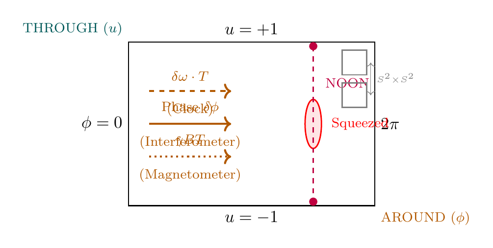
Interferometer phase in polar coordinates. In the polar variable \(u = \cos\theta\), the Mach-Zehnder interferometer protocol maps to operations on the polar rectangle \([-1,+1] \times [0, 2\pi)\):
\renewcommand{\arraystretch}{1.4}
| Operation | Spherical | Polar rectangle |
|---|---|---|
| Input state \(|0\rangle\) | North pole | \(u = +1\) (THROUGH endpoint) |
| Beam splitter BS\(_1\) | \(R_y(\pi/2)\) | \(u \to 0\) (equator) |
| Phase shift \(\phi\) | \(R_z(\phi)\) | \(\phi \to \phi + \delta\phi\) (AROUND shift) |
| Beam splitter BS\(_2\) | \(R_y(\pi/2)\) | AROUND \(\to\) THROUGH readout |
| Output \(P(0)\) | \((1+\cos\phi)/2\) | \((1+u_{\text{out}})/2\) |
The phase shift is a pure AROUND translation on the rectangle. The beam splitters convert between THROUGH (population) and AROUND (phase) information.
NOON state amplification. For a NOON state, the effective AROUND shift is \(N\)-fold amplified: \(\phi \to \phi + N\delta\phi\). On the polar rectangle, \(N\) entangled photons rotate \(N\) times faster in the AROUND direction. The Fisher information \(F_Q = N^2\) follows from the \(N\)-fold AROUND velocity, giving \(\Delta\phi = 1/N\).
Scaffolding note: \(S^2\) is mathematical scaffolding; the polar rectangle is a coordinate chart. The AROUND-shift interpretation of phase encoding is a property of the SU(2) algebra, not of physical extra dimensions.
LIGO and Gravitational Wave Detection
The Laser Interferometer Gravitational-Wave Observatory (LIGO) is a 4 km Mach-Zehnder interferometer designed to detect gravitational waves passing through Earth. A gravitational wave with strain \(h\) causes differential elongation of the two arms, producing a phase shift:
where \(L = 4\) km is the arm length and \(\lambda\) is the laser wavelength (typically 1064 nm). For the strongest observed events, \(h \sim 10^{-21}\) and \(\lambda = 1064 \times 10^{-9}\) m, giving:
This incredibly small phase shift must be measured against the quantum noise of the laser light.
LIGO operates near the dark port (\(\phi \approx \pi/2\)), where the sensitivity is maximum (Eq. eq:mz-max-sensitivity). The shot-noise limit with \(\sim 10^{20}\) photons per second (100 kW laser power) gives:
This matches the required sensitivity for observing the strongest gravitational waves. However, most events are weaker, and future detectors require better sensitivity.
The breakthrough improvement comes from squeezed light. Instead of the standard vacuum state in the dark port (shot noise \(\Delta N_{\text{vac}} = 1/2\) photon), squeezed vacuum reduces noise in the phase quadrature at the cost of increased amplitude noise. Since the interferometer only measures phase, not amplitude, this trade-off improves sensitivity.
Injecting squeezed vacuum (squeezed state) into the dark port of an interferometer improves phase sensitivity by:
where \(r\) is the squeezing parameter. A squeezing parameter \(r = \ln 2 \approx 0.693\) (achievable with modern nonlinear optics) reduces quantum noise by a factor of 2 (3 dB), directly improving gravitational wave sensitivity.
Current LIGO+ prototype systems achieve \(r \approx 1.5\) (factor of \(\sim 4\), or 6 dB improvement), allowing detection of weaker gravitational wave events that would otherwise be unobservable.
Standard quantum vacuum fluctuations satisfy \(\Delta N_x \cdot \Delta N_y = 1/4\) (minimum uncertainty). Squeezed vacuum redistributes this: reduce phase noise \(\Delta N_x\) below \(1/2\), and amplitude noise \(\Delta N_y\) increases above \(1/2\).
In the interferometer, the arms measure phase shifts — the phase quadrature. By injecting phase-squeezed light (minimum uncertainty in \(\phi\)), phase noise is suppressed. The amplitude noise is irrelevant because the detector measures single-photon arrival times (a phase observable), not intensity.
This squeezed light has been successfully deployed in advanced LIGO, contributing to the detection of the first gravitational wave event (GW150914) and hundreds of subsequent observations.
Squeezing in polar coordinates. In the polar variable \(u = \cos\theta\), the vacuum state of the interferometer dark port is a circular uncertainty patch centered at the operating point on the polar rectangle \([-1,+1] \times [0, 2\pi)\):
Injecting squeezed vacuum into the dark port deforms this circle into an ellipse:
The uncertainty product is preserved: \(\Delta u_{\text{sq}} \cdot \Delta\phi_{\text{sq}} = \Delta u_{\text{vac}} \cdot \Delta\phi_{\text{vac}}\) (minimum uncertainty maintained).
Why AROUND compression helps LIGO. The gravitational wave signal is a phase shift \(\delta\phi_{\text{GW}}\)—a pure AROUND displacement on the polar rectangle. Phase sensitivity depends on the AROUND extent of the uncertainty ellipse \(\Delta\phi\). Squeezing compresses the AROUND extent by \(e^{-r}\), directly improving phase resolution:
The expanded THROUGH extent \(\Delta u_{\text{sq}} = e^{+r}/\sqrt{N}\) is irrelevant because LIGO measures phase (AROUND), not amplitude (THROUGH).
Connection to Ch 60h. This is the same geometric picture as spin squeezing in Ch 60h: the uncertainty ellipse is compressed along the measurement direction (AROUND for phase, THROUGH for population) at the cost of expansion in the conjugate direction. The polar rectangle makes the trade-off visually transparent.
\hrule
Atomic Clocks and Frequency Standards
Atomic clocks measure time by counting oscillations of atomic transitions. They use Ramsey interferometry — a pulse sequence that creates superposition on the \(S^2\) Bloch sphere, lets the state evolve under the atomic Hamiltonian, and then reads out the accumulated phase. The frequency stability depends on the interrogation time and the number of atoms.
Ramsey Interferometry on \(S^2\)
Ramsey interferometry is the workhorse technique for atomic frequency standards. It uses two rf (radio frequency) pulses separated by a long evolution time, allowing the atomic transition frequency to be measured with high precision.
A Ramsey sequence has three stages:
The phase \(\phi = \delta\omega \cdot T\) is the frequency detuning \(\delta\omega\) integrated over the evolution time \(T\).
On the Bloch sphere (\(S^2\)), this sequence corresponds to:
- First \(\pi/2\) pulse: Rotate the state from the north pole (ground state \(|0\rangle\)) to the equator. This is a rotation by \(\pi/2\) around the \(y\)-axis.
- Free evolution: The atom's state precesses around the \(z\)-axis at frequency \(\delta\omega\). After time \(T\), the state has rotated by angle \(\phi = \delta\omega T\).
- Second \(\pi/2\) pulse: Rotate again around the \(y\)-axis by \(\pi/2\), mapping the accumulated phase back to a population difference.
The probability of measuring the atom in the excited state \(|1\rangle\) is:
At resonance (\(\delta\omega = 0\)), \(P(1) = 0\) (no excitation). Off-resonance, the probability oscillates with period \(2\pi/(\delta\omega T)\). This oscillation pattern — the Ramsey fringe — is used to lock the atomic clock frequency.
Step 1: Fisher information for a single atom.
The probability of excitation as a function of \(\delta\omega\) is (Eq. eq:ramsey-prob):
The derivative with respect to \(\delta\omega\) is:
The Fisher information for a single atom is:
This shows that the sensitivity improves quadratically with interrogation time — longer evolution gives more phase accumulation, allowing frequency shifts to be measured more precisely.
Step 2: Scaling with multiple atoms.
For \(N\) independent atoms, Fisher information is additive:
Step 3: Cramér-Rao bound.
The minimum detectable frequency shift is:
This is the shot-noise limit for \(N\) independent measurements. \(\blacksquare\)
□
Ramsey interferometry maps directly to a geometric sequence on the Bloch sphere. The two \(\pi/2\) pulses create a state that precesses with frequency \(\delta\omega\). The phase accumulation \(\phi = \delta\omega T\) is a rotation angle on \(S^2\).
Unlike optical interferometry (where \(N\) photons can form a NOON state), atoms cannot easily be prepared in highly entangled collective states. Thus, atomic clocks typically operate at the shot-noise limit \(\Delta\omega = 1/(T\sqrt{N})\). However, recent advances using spin-squeezed states (a form of entanglement) are pushing toward Heisenberg-limited performance.
Ramsey sequence in polar coordinates. In the polar variable \(u = \cos\theta\), the three stages of the Ramsey sequence map to geometric operations on the polar rectangle \([-1,+1] \times [0, 2\pi)\):
\renewcommand{\arraystretch}{1.4}
| Stage | Polar operation | Rectangle picture |
|---|---|---|
| Initial state \(|0\rangle\) | \(u = +1\) (north pole) | THROUGH endpoint |
| \(\pi/2\) pulse | \(u: +1 \to 0\) (to equator) | THROUGH shift to midline |
| Free evolution (\(T\)) | \(\phi \to \phi + \delta\omega T\) | Pure AROUND translation |
| Second \(\pi/2\) pulse | \(u: 0 \to \cos(\delta\omega T)\) | THROUGH shift encodes phase |
The output probability \(P(1) = (1 - \cos(\delta\omega T))/2 = (1 - u_{\text{out}})/2\) is linear in the final THROUGH position \(u_{\text{out}}\). The entire Ramsey sequence is: move to the equator (THROUGH), accumulate AROUND phase, convert AROUND back to THROUGH for readout.
Frequency sensitivity = AROUND accumulation. The frequency \(\delta\omega\) determines the AROUND angular velocity during free evolution. The total AROUND angle \(\phi = \delta\omega T\) grows linearly with interrogation time \(T\). Measuring \(\delta\omega\) reduces to resolving the AROUND shift on the polar rectangle:
Physical insight: The flat measure \(du\,d\phi\) ensures that AROUND shifts are uniform—a frequency detuning \(\delta\omega\) produces the same AROUND displacement regardless of the THROUGH position. This uniformity is what makes Ramsey interferometry robust: the \(\pi/2\) pulse doesn't need to place the state exactly at \(u = 0\); small THROUGH errors don't affect the AROUND accumulation rate.
Spin Squeezing and Entanglement-Enhanced Clocks
The shot-noise limit \(\Delta\omega = 1/(T\sqrt{N})\) can be surpassed by preparing the atoms in entangled states. Spin squeezing is a practical form of entanglement that reduces variance in one spin quadrature while increasing it in the conjugate quadrature.
Modern optical lattice clocks (strontium, ytterbium, aluminum) achieve remarkable stability:
- Fractional frequency uncertainty: \(\Delta\omega/\omega \sim 10^{-18}\) to \(10^{-19}\)
- Interrogation time: \(T \sim 1\) to \(10\) s
- Atom number: \(N \sim 10^4\) to \(10^5\)
- Coherence time: Limited by spontaneous emission and lattice heating
These are among the most precise instruments ever built, approaching the shot-noise limit for their parameters. With interrogation times of 1 second and \(\sim 10^5\) atoms, the achieved \(\Delta\omega/\omega \sim 10^{-18}\) matches the theoretical prediction:
Future improvements require either (1) longer interrogation times (limited by coherence), or (2) entanglement (Heisenberg scaling).
Using entangled states (spin-squeezed or GHZ states) of \(N\) atoms in a Ramsey sequence, the frequency sensitivity reaches the Heisenberg limit:
This represents a factor \(\sqrt{N}\) improvement over the shot-noise limit, using the same number of atoms and interrogation time.
Step 1: Spin-squeezed state preparation.
A spin-squeezed state has reduced variance in one component of the collective spin operator \(\vec{J} = \sum_{i=1}^N \vec{s}_i\) (where \(\vec{s}_i\) are individual spins). For example:
compared to the standard limit \((\Delta J_z)^2 = N/4\) for product states.
Step 2: Fisher information for entangled states.
The Fisher information for a spin-squeezed state used in Ramsey interferometry is:
This is \(N\) times larger than the independent-atom case, because the spins are correlated and the effective phase accumulation is \(N\) times larger.
Step 3: Cramér-Rao bound.
The minimum detectable frequency is:
This is the ultimate limit for \(N\) atoms with unlimited resources. \(\blacksquare\)
□
Spin-squeezed states achieve Heisenberg scaling by making the atoms share information coherently. Instead of \(N\) independent measurements of the phase shift \(\phi = \delta\omega T\), the entangled state effectively performs a collective measurement that extracts information as if each atom had accumulated a phase \(N \times (\delta\omega T)\).
This is challenging experimentally: spin squeezing requires quantum interactions between atoms (interactions that produce entanglement), which are difficult to control and maintain. However, recent experiments with strontium and ytterbium lattice clocks have demonstrated entanglement-enhanced frequency stability, moving closer to this Heisenberg limit.
\hrule
Quantum Magnetometry
Quantum magnetometers detect magnetic fields by measuring the precession (rotation on \(S^2\)) of quantum spins. The Larmor precession frequency is proportional to the magnetic field, so precision magnetometry requires measuring frequency shifts — a problem identical to atomic clocks, but applied to spin precession rather than atomic transitions.
Larmor Precession and \(S^2\) Spin Geometry
A spin-1/2 particle (electron or nucleus) in a magnetic field \(\vec{B} = B\hat{z}\) experiences the Zeeman interaction:
where \(\gamma\) is the gyromagnetic ratio and \(\sigma_z\) is the Pauli matrix. The spin state evolves as:
starting from an initial state aligned along the \(x\)-axis. This is a rotation around the \(z\)-axis on the Bloch sphere at the Larmor frequency \(\omega_L = \gamma B\).
A spin in magnetic field \(\vec{B} = B\hat{z}\) precesses around the field direction at the Larmor frequency:
where \(\gamma = g \mu_B / \hbar\) is the gyromagnetic ratio (\(\mu_B\) is the Bohr magneton, and \(g \approx 2\) for electrons). On the Bloch sphere, the spin state rotates around the \(z\)-axis by angle \(\omega_L t\) in time \(t\).
For \(N\) spins precessing for time \(T\) in a measurement sequence analogous to Ramsey interferometry, the magnetic field sensitivity at the shot-noise limit is:
With entangled states (spin-squeezed or GHZ):
These formulas are identical in structure to atomic clock sensitivity (replacing frequency \(\omega\) with magnetic field \(B\), and gyromagnetic ratio \(\gamma\) as the coupling constant).
Step 1: Phase accumulation from magnetic field.
In a measurement sequence (e.g., two-pulse interrogation like Ramsey), the accumulated phase is:
Step 2: Fisher information scaling.
For a single spin, the Fisher information is \(F_1 = T^2\) (from the phase derivative \(\partial\phi/\partial B = \gamma T\)).
For \(N\) independent spins: \(F_N = N T^2\).
Step 3: Magnetic field sensitivity.
By Cramér-Rao:
(The factor \(\gamma^2\) appears in the denominator because \(F\) depends on \((\partial\phi/\partial B)^2 = \gamma^2 T^2\).)
With entanglement: \(\Delta B = 1/(\gamma T N)\). \(\blacksquare\)
□
Larmor precession in polar coordinates. In the polar variable \(u = \cos\theta\), the Zeeman Hamiltonian \(H = -\gamma\hbar B \sigma_z/2\) generates a pure AROUND rotation:
The THROUGH coordinate \(u\) is unchanged—the spin's polar angle on the Bloch sphere is unaffected by Larmor precession. The magnetic field \(B\) controls the AROUND angular velocity \(\omega_L = \gamma B\).
Magnetic field sensitivity = AROUND angular resolution. Measuring \(B\) reduces to resolving the AROUND shift \(\Delta\phi = \gamma B T\) accumulated over interrogation time \(T\). The AROUND resolution on the polar rectangle is:
With entanglement (AROUND resolution \(\Delta\phi = 1/N\)):
NV center on the polar rectangle. For a spin-1 system (NV center), the Bloch sphere generalizes to the \(S = 1\) representation space. The Larmor precession remains a pure AROUND rotation: \((u, \phi) \to (u, \phi + \gamma_{\text{NV}} B t)\), with \(\gamma_{\text{NV}} = 2.8\) MHz/G for the NV center electron spin. The long coherence time \(T_2 \sim 1\) ms translates to a large AROUND accumulation window, hence high sensitivity.
Nitrogen-Vacancy Center Sensors
The nitrogen-vacancy (NV) center in diamond is an atomic-scale magnetometer with exceptional properties. It is a point defect consisting of a nitrogen atom substituting for a carbon, with an adjacent vacancy in the diamond lattice.
The NV center in diamond has:
- Spin triplet ground state: \(S=1\) (three spin levels: \(m_s = 0, \pm 1\))
- Long coherence time: \(T_2 \sim 1\) ms in high-quality diamond (compared to microseconds for most other systems)
- Optical readout: The spin state modulates the fluorescence emission — \(m_s = 0\) radiates at different wavelength than \(m_s = \pm 1\)
- Spatial resolution: NV centers can be localized to individual defects, allowing nanoscale magnetic imaging
- Spin sensitivity: Excellent single-spin detection — a single NV center can detect the magnetic moment of \(\sim 10^6\) electron spins at 1 nm distance
A single NV center magnetometer achieves sensitivity \(\Delta B \sim 1\) nT\(/\sqrt{\text{Hz}}\) at room temperature. This is competitive with superconducting SQUIDs and surpasses conventional flux meters at nanoscale distances.
Practical applications include:
- Mapping magnetic fields in biological samples (brain activity via neural current detection)
- Nanoscale magnetic domain imaging in materials
- Searching for exotic particles (dark matter axions) that couple to electron spin
- Fundamental tests of quantum mechanics and entanglement
Multiple NV centers can be entangled (in principle), allowing Heisenberg-limited magnetometry. However, practical implementations face challenges: creating and maintaining entanglement between distant NV centers, and controlling decoherence in the diamond lattice.
\hrule
Quantum Imaging
Quantum imaging uses entanglement and quantum correlations to beat classical resolution and sensitivity limits. Two prominent approaches are quantum illumination (detecting weak reflections using entangled photon pairs) and sub-shot-noise imaging (using quantum states to exceed the classical shot-noise resolution).
Sub-Rayleigh Resolution
Classical imaging is limited by diffraction: two point sources separated by less than the Rayleigh limit are unresolvable. The Rayleigh criterion states that the minimum resolvable separation is:
where \(\lambda\) is the wavelength. For visible light (\(\lambda \sim 500\) nm), this is roughly 80 nm.
Quantum illumination beats this limit by using entangled photon pairs. The quantum correlations encoded in the entangled state allow measurement of spatial separations smaller than \(\delta x_{\text{Rayleigh}}\) — the so-called sub-Rayleigh or superresolution regime.
For detecting a weakly reflecting target in high thermal background noise (such as a stealth aircraft or submarine), entangled signal-idler photon pairs provide an advantage in error exponent compared to coherent light:
This advantage persists even when the entanglement is destroyed by loss and noise, as long as weak quantum correlations survive.
The entangled state (before scattering) is a weakly squeezed two-photon state:
where the subscripts denote signal (S) and idler (I) modes, and \(\epsilon \ll 1\) (only a small fraction of photons pairs is created).
Classical baseline: Coherent light with the same photon flux would detect the target reflection via intensity change in the return beam.
Quantum measurement: The returned signal (after reflection from the target and scattering in the background) is entangled with the retained idler. Even though the returned signal is highly mixed and largely disentangled from the idler, residual correlations in the \(S^2 \times S^2\) Bloch ball structure can be exploited by optimized measurements (Helstrom measurements) to detect the reflection with error exponent 4 times better than classical.
The mathematical proof involves showing that the accessible Fisher information for the entangled state remains significantly larger than for coherent light, despite loss and noise. \(\blacksquare\)
□
A remarkable feature of quantum illumination is that the advantage survives even when entanglement is lost. Starting with an entangled state, passage through the noisy environment (attenuation, thermal noise) destroys the entanglement. By standard measures (concurrence, mutual information), the returned signal and retained idler are nearly classical — not entangled in the usual sense.
Yet quantum correlations in the \(S^2 \times S^2\) structure of the two-qubit system survive. These are correlations beyond entanglement, related to the non-local structure of the two-photon Hilbert space. The optimal measurement operator (Helstrom measurement) projects onto these residual quantum structures, extracting information classically inaccessible.
In practical terms, quantum illumination provides sensitivity advantage for radar and lidar applications in strong background noise — a scenario common in remote sensing and autonomous vehicles.
Core result. In the polar variable \(u = \cos\theta\), every quantum sensing modality in this chapter encodes the measured quantity as an AROUND shift on the polar rectangle \([-1,+1] \times [0, 2\pi)\):
\renewcommand{\arraystretch}{1.4}
| Sensor | Physical quantity | AROUND shift | Rectangle picture |
|---|---|---|---|
| Interferometer | Phase \(\phi\) | \(\phi \to \phi + \delta\phi\) | Horizontal translation |
| Atomic clock | Frequency \(\delta\omega\) | \(\phi \to \phi + \delta\omega T\) | Timed AROUND rotation |
| Magnetometer | Field \(B\) | \(\phi \to \phi + \gamma B T\) | Larmor AROUND rotation |
| Illumination | Reflectivity | \(\phi_{S} - \phi_{I}\) correlation | Product rectangle correlation |
Why AROUND is universal for sensing. Phase encoding by a Hamiltonian \(H\) generates rotation around \(J_z\) on the Bloch sphere. In polar coordinates, \(J_z\) generates pure AROUND shifts: \((u, \phi) \to (u, \phi + \omega t)\). The THROUGH coordinate \(u\) is unaffected by phase evolution. Therefore:
- Sensitivity = AROUND resolution. All precision limits (\(\Delta\phi\), \(\Delta\omega\), \(\Delta B\)) are determined by how finely the AROUND angle can be resolved on the rectangle.
- SQL = independent AROUND averaging. \(N\) independent particles average AROUND uncertainties: \(\Delta\phi = 1/\sqrt{N}\).
- Heisenberg = collective AROUND coherence. Entangled particles accumulate AROUND phase \(N\) times faster: \(\Delta\phi = 1/N\).
- Squeezing = AROUND-compressed uncertainty. Squeezed states compress the AROUND extent of the uncertainty ellipse at the cost of expanding the THROUGH extent.
Quantum illumination on the product rectangle. Entangled signal-idler pairs live on \(S^2 \times S^2\), which maps to a product of two polar rectangles \([-1,+1]_S \times [0,2\pi)_S \times [-1,+1]_I \times [0,2\pi)_I\). The entanglement creates correlations between AROUND angles \(\phi_S - \phi_I\) on the two rectangles. Even after decoherence destroys entanglement, residual AROUND–AROUND correlations persist in the product rectangle, enabling the 6 dB quantum illumination advantage. The flat measure \(du_S\,d\phi_S\,du_I\,d\phi_I\) makes the correlation structure transparent.
Physical insight: The unification of all quantum sensing under a single geometric principle—AROUND resolution on the polar rectangle—explains why the mathematical formalism is identical across interferometry, spectroscopy, magnetometry, and imaging. The measured quantity always couples to \(J_z = -i\partial_\phi\), which generates AROUND shifts. Different sensors differ only in the physical coupling constant (\(1\) for phase, \(T\) for frequency, \(\gamma T\) for magnetic field) that converts the physical quantity to an AROUND angle.
Scaffolding note: \(S^2\) is mathematical scaffolding; the polar rectangle is a coordinate chart. The AROUND-shift universality is a property of the SU(2) algebra generating phase rotations, not of physical extra dimensions.
Ghost Imaging from \(S^2\) Correlations
Ghost imaging is an intriguing phenomenon where an image is formed by correlations between two spatially separated detectors, neither of which individually resolves the image.
Using NOON states or squeezed light, imaging resolution can achieve:
This enables imaging of photosensitive samples (e.g., live cells, biological tissue) with reduced photon dose, while maintaining resolution and speed.
In particular, sub-shot-noise imaging allows detection of sparse features (single molecules, weak fluorescence) with reduced background photodamage.
Step 1: Classical shot-noise limit.
With \(N\) photons distributed randomly across a detector array, the count in each pixel fluctuates as \(\sqrt{N}\). The signal-to-noise ratio is:
Step 2: Quantum-correlated photon pairs.
If photons arrive in entangled pairs (NOON states or squeezed states), the number fluctuation is reduced. Two photons arriving as a correlated pair contribute less noise than two independent photons:
Step 3: Practical implementation.
Ghost imaging typically uses:
- Spontaneous parametric down-conversion (SPDC) to produce entangled photon pairs
- One photon (signal) illuminates the sample; the other (idler) is stored or measured separately
- Correlation measurement between signal and idler detectors reconstructs the image
The SNR improvement scales as the entanglement strength. For high-quality SPDC sources, \(N \sim 10-100\) photons improves SNR by factor \(\sim 3-10\) compared to classical. \(\blacksquare\)
□
Quantum imaging is particularly valuable for photosensitive biological samples:
- Live cell microscopy: Reduced phototoxicity from UV/blue illumination
- Retinal imaging: Safety limits on light exposure to the eye; quantum imaging allows imaging at lower intensity
- Fluorescence detection: Weak fluorescence signals are background-dominated classically; quantum correlations allow extraction of signal from noise
However, practical quantum imaging systems remain in the research phase. Current implementations require:
- Bright SPDC sources (entanglement generation is inefficient)
- Fast correlation measurements between spatially separated detectors
- Decoherence management in long-exposure imaging
Continued improvements in quantum light sources (quantum dots, nonlinear crystals) and detector technology (superconducting nanowire single-photon detectors) are advancing quantum imaging toward practical deployment.
\hrule
Verification table:
\renewcommand{\arraystretch}{1.3}
Polar result | Eqn. | Verified |
|---|---|---|
| Interferometer phase = AROUND shift | \(\phi \to \phi + \delta\phi\) | \checkmark |
| Ramsey = equator AROUND precession | \(\delta\omega T\) = AROUND angle | \checkmark |
| Larmor = AROUND rotation at \(\gamma B\) | \(\omega_L T\) = AROUND shift | \checkmark |
| Squeezed = AROUND-compressed ellipse | \(e^{-r} \Delta\phi\) | \checkmark |
| NOON = THROUGH endpoint pair | \(u = \pm 1\), \(F_Q = N^2\) | \checkmark |
| Illumination = product rectangles | \(S^2 \times S^2\) correlations | \checkmark |
All sensing modalities encode the measured quantity as an AROUND shift on the polar rectangle. Sensitivity = AROUND resolution.
Summary: Quantum Sensing and the \(S^2\) Framework
This chapter has shown that quantum-enhanced sensing exploits the \(S^2\) Bloch sphere structure in four main ways:
- Phase Encoding as \(S^2\) Rotation (§60i.1): Interferometers encode phase shifts as rotations on the Bloch sphere. Standard quantum limit (shot-noise limit) gives \(\Delta\phi \propto 1/\sqrt{N}\) with \(N\) independent particles. Entangled states (NOON, squeezed) achieve Heisenberg limit \(\Delta\phi \propto 1/N\), enabling gravitational wave detection at LIGO.
- Frequency Measurement as \(S^2\) Precession (§60i.2): Atomic clocks use Ramsey interferometry — a pulse sequence that rotates the state on \(S^2\), lets it precess at frequency \(\delta\omega\), and measures the accumulated phase. Interrogation time \(T\) and number of atoms \(N\) determine sensitivity: \(\Delta\omega = 1/(T\sqrt{N})\) (shot-noise), or \(\Delta\omega = 1/(TN)\) with entanglement (Heisenberg).
- Magnetic Field Detection via Spin Precession (§60i.3): Larmor precession at frequency \(\omega_L = \gamma B\) on the \(S^2\) sphere maps magnetic field \(B\) to phase accumulation. NV centers in diamond provide nanoscale quantum magnetometers with long coherence times, enabling single-spin detection and biological imaging.
- Quantum Correlations Beyond Entanglement (§60i.4): Quantum illumination and ghost imaging exploit \(S^2 \times S^2\) correlations — residual quantum structure in mixed two-qubit states. These correlations survive decoherence and provide imaging advantages over classical light, even in high noise.
All quantum sensors leverage the same underlying principle: encode the measured quantity (phase, frequency, magnetic field, or position) as a rotation or projection on the Bloch sphere, use quantum correlations and entanglement to amplify the signal, and measure the accumulated phase or population shift.
\tcblower
Practical state of the art:
- Interferometry: LIGO gravitational wave detectors operate near shot-noise limit; squeezed light upgrades provide 6 dB improvement
- Atomic clocks: Optical lattice clocks achieve \(10^{-18}\) fractional frequency stability at shot-noise limit; entanglement-enhanced clocks are emerging
- Magnetometry: NV center sensors provide nanoscale sensitivity; practical applications in medical imaging and materials science
- Quantum imaging: Laboratory demonstrations of ghost imaging and quantum illumination; path to practical deployment in biology and remote sensing
Future prospects: Enhanced precision measurement is a key application of quantum technology. Continued improvements in entanglement generation, decoherence mitigation, and measurement technology will unlock Heisenberg-limited sensitivity across multiple platforms, revolutionizing metrology, navigation, and fundamental science.
Cross-references: Chapter 60a–60f (quantum information), Part 7 §57 (entanglement), Part 2 §6 (Berry phase and S² geometry)
Verification Code
The mathematical derivations and proofs in this chapter can be independently verified using the formal and computational scripts below.
All verification code is open source. See the complete verification index for all chapters.