Chapter 124

The Aggregate Certainty Theorem

Introduction

The Temporal Determination Theorem (Chapter 90) established that probability distributions over future aggregate events are geometric consequences of P1. This chapter proves the complementary result: as the number of particles $N$ grows, aggregate observables become deterministic—their fluctuations vanish exponentially.

This is the Aggregate Certainty Theorem, which provides the mathematical foundation for why collective properties can be predicted even though individual outcomes cannot. The result follows from concentration of measure on the product space $(S^2)^N$, which is itself a consequence of the positive curvature of $S^2$ and the derived natural measure of Chapter 88.

Scaffolding Interpretation

The Aggregate Certainty Theorem operates at the interface between $S^2$ scaffolding and 4D physics. The concentration bound arises from the geometry of $S^2$ (scaffolding), but its physical consequence—macroscopic determinism—is a 4D observable prediction.

Averaging Over Futures

Concentration of Measure

Definition 124.10 (Concentration of Measure)

A probability measure $\mu$ on a space $X$ exhibits concentration of measure if, for typical Lipschitz functions $f : X \to \mathbb{R}$:

$$ P(|f - \langle f \rangle| > \varepsilon) \ll 1 $$ (124.1)

and this probability decreases rapidly with the “size” of $X$ (e.g., dimension or particle number).

The key intuition is that in high-dimensional spaces, “most” of the measure is concentrated near the average value of any sufficiently smooth function. Extreme values become exponentially rare as the dimension grows.

Lévy's Lemma on $S^2$

The starting point is a classical result from geometric measure theory, applied to the specific geometry of $S^2$.

Lemma 124.7 (Lévy's Lemma for $S^2$)

Let $f : S^2 \to \mathbb{R}$ be a function with Lipschitz constant $L$:

$$ |f(\Omega) - f(\Omega')| \leq L \cdot d(\Omega, \Omega') $$ (124.2)

where $d$ is the geodesic distance on $S^2$. Then:

$$ \mu\!\left(\left\{|f - \langle f \rangle| > \varepsilon \right\}\right) \leq 2\exp\!\left(-\frac{\varepsilon^2}{2L^2}\right) $$ (124.3)

Proof.

This is a standard result in geometric measure theory. The derivation proceeds in three steps:

Step 1: The uniform measure on $S^2$ satisfies a log-Sobolev inequality. For the sphere of radius $r$, the log-Sobolev constant is $\rho_{\mathrm{LS}} = 1/(r^2)$, which for the unit sphere gives $\rho_{\mathrm{LS}} = 1$.

Step 2: By Herbst's argument, the log-Sobolev inequality implies sub-Gaussian concentration. Specifically, for any Lipschitz function $f$ with constant $L$:

$$ \mathbb{E}[e^{\lambda(f - \mathbb{E}[f])}] \leq e^{\lambda^2 L^2 / (2\rho_{\mathrm{LS}})} $$ (124.4)

Step 3: Applying the Chernoff bound (optimizing over $\lambda$) yields the stated concentration inequality.

The positive Ricci curvature of $S^2$ ($\mathrm{Ric} = 1/r^2$) is the geometric origin of the concentration phenomenon. (See: Ledoux (2001), Theorem 5.1) □ □

Extension to Product Spaces

Theorem 124.1 (Concentration on $(S^2)^N$)

For a function $F : (S^2)^N \to \mathbb{R}$ with Lipschitz constant $L$ in the product metric:

$$ P\!\left(|F - \langle F \rangle| > \varepsilon\right) \leq 2\exp\!\left(-\frac{N\varepsilon^2}{2L^2}\right) $$ (124.5)

Proof.

For product measures, concentration “tensorizes”: if each factor exhibits concentration with a given parameter, the product exhibits enhanced concentration proportional to $N$.

Step 1: The product measure on $(S^2)^N$ is:

$$ d\mu_N = \prod_{i=1}^N \frac{d\Omega_i}{4\pi} $$ (124.6)

Step 2: Each $S^2$ factor satisfies Lévy's lemma (Lemma lem:P12-Ch91-levy) with log-Sobolev constant $\rho_{\mathrm{LS}} = 1$.

Step 3: By the tensorization property of log-Sobolev inequalities (Ledoux, Theorem 5.7), the product space has log-Sobolev constant:

$$ \rho_{\mathrm{LS}}^{(N)} = N \times \rho_{\mathrm{LS}}^{(1)} = N $$ (124.7)

Step 4: Repeating the Herbst–Chernoff argument with the enhanced log-Sobolev constant gives the stated bound with the factor of $N$ in the exponent. □ □

The factor of $N$ in the exponent is the crucial feature: concentration improves exponentially with particle number.

Polar Field Form of Product Concentration

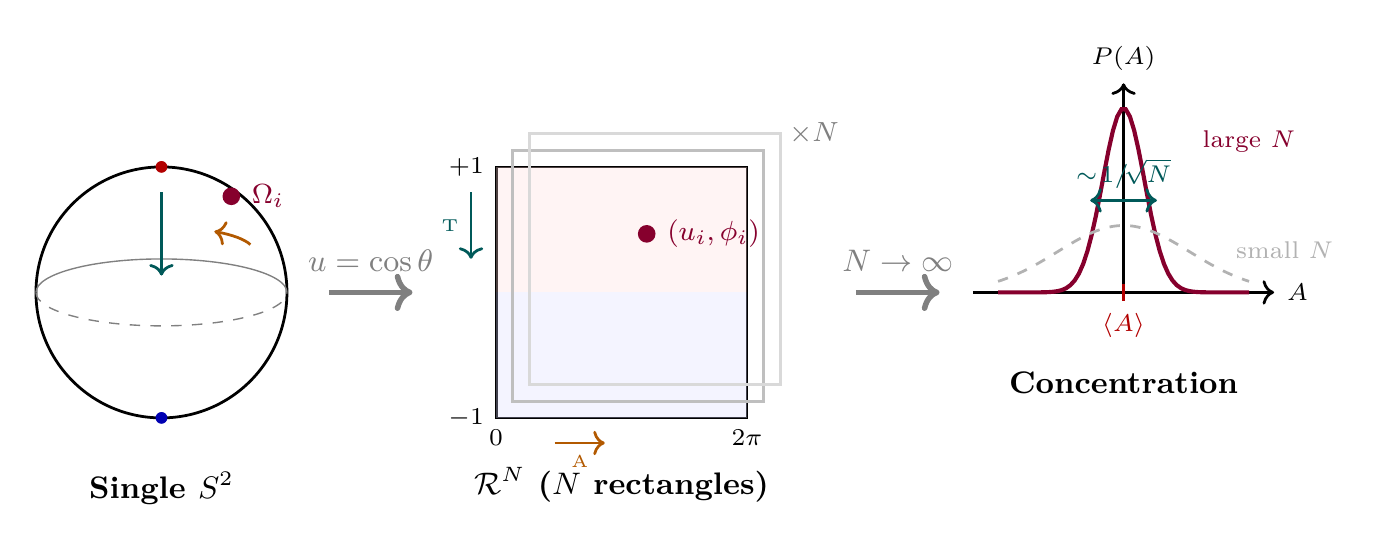
The concentration on $(S^2)^N$ becomes geometrically transparent in the polar field variable $u = \cos\theta$. Each $S^2$ factor maps to a flat rectangle $\mathcal{R} = [-1,+1] \times [0,2\pi)$, so the product space becomes:

$$ (S^2)^N \;\longleftrightarrow\; \mathcal{R}^N = [-1,+1]^N \times [0,2\pi)^N $$ (124.8)

The product measure of Eq. eq:ch91-product-measure takes the explicit form:

$$ d\mu_N = \prod_{i=1}^N \frac{du_i\, d\phi_i}{4\pi} $$ (124.9)

which is flat Lebesgue measure on $\mathcal{R}^N$. Each factor $du_i\,d\phi_i/(4\pi)$ is the uniform probability density on a single rectangle, normalized by the total area $4\pi = 2 \times 2\pi$ (THROUGH range $\times$ AROUND period).

The tensorization that drives concentration (Eq. eq:ch91-tensorization) is now manifest: flat rectangles tensorize trivially, and the log-Sobolev constant scales as $N$ because each independent rectangle contributes additively. The concentration bound becomes:

$$ P\!\left(|F - \langle F \rangle| > \varepsilon\right) \leq 2\exp\!\left(-\frac{N\varepsilon^2}{2L^2}\right) $$ (124.10)

where the Lipschitz constant $L$ is measured in the geodesic metric inherited from the $S^2$ metric $h_{ij}\,d\xi^i d\xi^j = R^2[du^2/(1-u^2) + (1-u^2)\,d\phi^2]$. The crucial point: the measure is flat ($du\,d\phi$), but the distance retains the curvature of $S^2$ through $h_{uu} = R^2/(1-u^2)$, and it is this curvature that generates concentration.

For functions that factorize into THROUGH and AROUND components, $F(\{u_i,\phi_i\}) = G(\{u_i\}) \cdot H(\\phi_i$\), the concentration decomposes:

$$ \text{Total concentration} = \underbrace{\text{THROUGH concentration} \vphantom{\int}}_{\text{$N$ independent $u_i \in [-1,+1]$}} \;\times\; \underbrace{\text{AROUND concentration} \vphantom{\int}}_{\text{$N$ independent $\phi_i \in [0,2\pi)$}} $$ (124.11)

Property	Spherical $(\theta, \phi)$	Polar $(u, \phi)$
Single-particle space	$S^2$ (curved)	$\mathcal{R} = [-1,+1] \times [0,2\pi)$ (flat measure)
$N$-particle space	$(S^2)^N$	$\mathcal{R}^N$ ($N$ independent rectangles)
Measure	$\prod d\Omega_i/(4\pi)$	$\prod du_i\,d\phi_i/(4\pi)$ (flat Lebesgue)
Area per particle	$4\pi$	$2 \times 2\pi$ (THROUGH $\times$ AROUND)
Determinant	$\sqrt{\det h} = R^2 \sin\theta$ (variable)	$\sqrt{\det h} = R^2$ (constant)
Tensorization	Abstract (log-Sobolev)	Manifest (flat $\times$ flat = flat)
Concentration source	Positive Ricci curvature	Curvature in $h_{uu} = R^2/(1-u^2)$ (metric, not measure)

The polar form reveals a key structural insight: concentration of measure on $(S^2)^N$ is not driven by curvature of the measure (which is flat in polar coordinates) but by curvature of the metric (which determines the Lipschitz condition). The distinction between flat measure and curved distance is invisible in spherical coordinates but transparent in the polar field variable.

Scaffolding Interpretation

Scaffolding note: The polar field variable $u = \cos\theta$ is a coordinate choice, not a new physical assumption. The product space $\mathcal{R}^N = [-1,+1]^N \times [0,2\pi)^N$ is the same mathematical object as $(S^2)^N$; the flat-rectangle picture is a representation that makes tensorization manifest. The physical conclusion—aggregate certainty with exponential concentration—follows identically in both coordinate systems.

**Figure 124.1:** Aggregate certainty in polar field coordinates. **Left:** A single particle's $S^2$ configuration maps to a point $(u_i, \phi_i)$ on the flat polar rectangle $\mathcal{R}$. **Center:** $N$ particles occupy $N$ independent rectangles; the product measure $\prod du_i\,d\phi_i/(4\pi)$ is flat Lebesgue on $\mathcal{R}^N$. **Right:** As $N$ grows, aggregate observables concentrate around their mean with width $\sim 1/\sqrt{N}$—the dashed curve (small $N$) sharpens into the solid curve (large $N$). Concentration is exponential in $N$.

Certainty from Indeterminacy

Statement of the Aggregate Certainty Theorem

Theorem 124.2 (The Aggregate Certainty Theorem)

Let $A : \mathcal{F}_t \to \mathbb{R}$ be an aggregate observable that:

Is symmetric under particle permutation.
Has Lipschitz constant $L$ with respect to the $S^2$ components.

Then:

$$ \boxed{P\!\left(|A - \langle A \rangle| > \varepsilon\right) \leq 2\exp\!\left(-\frac{N\varepsilon^2}{2L^2}\right)} $$ (124.12)

Consequently:

$$ \boxed{\lim_{N \to \infty} P\!\left(|A - \langle A \rangle| > \varepsilon\right) = 0} $$ (124.13)

for any fixed $\varepsilon > 0$.

Proof.

Step 1: Decompose the configuration space.

A configuration $\Sigma \in \mathcal{F}_t$ consists of spatial positions $\{x_i\}$ and $S^2$ configurations $\\Omega_i$. For fixed spatial positions, $A$ becomes a function on $(S^2)^N$.

Step 2: Apply concentration on $(S^2)^N$.

For fixed $\{x_i\}$, Theorem thm:P12-Ch91-product-concentration gives:

$$ P_{S^2}\!\left(|A - \langle A \rangle_{S^2}| > \varepsilon \;\middle|\; \{x_i\}\right) \leq 2\exp\!\left(-\frac{N\varepsilon^2}{2L^2}\right) $$ (124.14)

Step 3: Average over spatial positions.

The bound is independent of $\{x_i\}$ (it depends only on $N$, $\varepsilon$, and $L$), so averaging over the spatial measure preserves the bound:

$$ P\!\left(|A - \langle A \rangle| > \varepsilon\right) = \int P_{S^2}(\cdots \mid \{x_i\}) \, d\mu_{\mathrm{spatial}} \leq 2\exp\!\left(-\frac{N\varepsilon^2}{2L^2}\right) $$ (124.15)

Step 4: The limit.

As $N \to \infty$, the exponential $\exp(-N\varepsilon^2/(2L^2)) \to 0$ for any fixed $\varepsilon > 0$. □ □

Deterministic Aggregates

Corollary 124.8 (Deterministic Aggregates in the Thermodynamic Limit)

In the thermodynamic limit ($N \to \infty$):

$$ A(\Sigma) \xrightarrow{N \to \infty} \langle A \rangle \quad \text{(convergence in probability)} $$ (124.16)

Aggregate observables become deterministic.

Relative Fluctuations

Corollary 124.9 (Scaling of Relative Fluctuations)

For intensive observables (per-particle averages) $a = A/N$:

$$ \mathrm{Var}(a) = \frac{\mathrm{Var}(A)}{N^2} \sim \frac{1}{N} $$ (124.17)

Relative fluctuations scale as $1/\sqrt{N}$.

Proof.

For additive observables $A = \sum_i a_i$ with identical, independent contributions $a_i$:

$$ \mathrm{Var}(A) = N \cdot \mathrm{Var}(a_i) $$ (124.18)

Therefore, the relative standard deviation is:

$$ \frac{\mathrm{Std}(A)}{\langle A \rangle} = \frac{\sqrt{N \cdot \mathrm{Var}(a_i)}}{N \langle a_i \rangle} = \frac{1}{\sqrt{N}} \cdot \frac{\mathrm{Std}(a_i)}{\langle a_i \rangle} \sim \frac{1}{\sqrt{N}} $$ (124.19)

This is the standard $1/\sqrt{N}$ scaling of statistical mechanics, here derived from the geometric concentration bound. □ □

Derivation Chain Display

\dstep{P1: $ds_6^{\,2} = 0$ on $\mathcal{M}^4 \times S^2$}{Postulate}{Part 1} \dstep{$S^2$ has positive Ricci curvature}{Geometry of $S^2$}{Ch. 87} \dstep{Uniform measure on $S^2$ satisfies log-Sobolev inequality} {Curvature $\to$ log-Sobolev}{Ch. 88} \dstep{Lévy's lemma: exponential concentration on $S^2$} {Herbst argument}{This chapter} \dstep{Tensorization: concentration on $(S^2)^N$ with factor $N$} {Product log-Sobolev}{This chapter} \dstep{Aggregate Certainty Theorem: $P(|A - \langle A\rangle| > \varepsilon) \leq 2e^{-N\varepsilon^2/(2L^2)}$} {Spatial averaging}{This chapter} \dstep{Large-$N$ determinism: aggregates become certain} {$N \to \infty$ limit}{This chapter} \dstep{Polar verification: $d\mu_N = \prod du_i\,d\phi_i/(4\pi)$ flat Lebesgue on $\mathcal{R}^N$; tensorization manifest; concentration from metric curvature $h_{uu} = R^2/(1-u^2)$, not measure curvature} {Polar coordinate reformulation}{\Ssec:ch91-polar-product}

Macroscopic Determinism

The Psychohistory Threshold

Theorem 124.3 (Psychohistory Threshold)

To predict an aggregate observable $A$ with accuracy $\varepsilon$ (maximum deviation from mean) and confidence $1 - \delta$ (probability of success), the minimum number of particles required is:

$$ \boxed{N_{\min} = \frac{2L^2}{\varepsilon^2} \ln\frac{2}{\delta}} $$ (124.20)

Proof.

We require:

$$ P(|A - \langle A \rangle| > \varepsilon) \leq \delta $$ (124.21)

From the Aggregate Certainty Theorem (Theorem thm:P12-Ch91-aggregate-certainty):

$$ 2\exp\!\left(-\frac{N\varepsilon^2}{2L^2}\right) \leq \delta $$ (124.22)

Solving for $N$:

$$\begin{aligned} \exp\!\left(-\frac{N\varepsilon^2}{2L^2}\right) &\leq \frac{\delta}{2} \\ -\frac{N\varepsilon^2}{2L^2} &\leq \ln\frac{\delta}{2} \\ N &\geq \frac{2L^2}{\varepsilon^2} \ln\frac{2}{\delta} \end{aligned}$$ (124.31)

□ □

Numerical Examples

Example 1: Thermodynamic prediction. For a gas with normalized Lipschitz constant $L = 1$, requiring 1% accuracy ($\varepsilon = 0.01$) at 99% confidence ($\delta = 0.01$):

$$ N_{\min} = \frac{2 \times 1}{(0.01)^2} \times \ln\!\left( \frac{2}{0.01}\right) = 20{,}000 \times 5.3 \approx 1.06 \times 10^5 $$ (124.23)

Systems with $N > 10^5$ particles are predictable to 1% with 99% confidence.

Example 2: High-precision prediction. For 0.1% accuracy ($\varepsilon = 0.001$) at 99.9% confidence ($\delta = 0.001$):

$$ N_{\min} = \frac{2}{(0.001)^2} \times \ln\!\left( \frac{2}{0.001}\right) = 2 \times 10^6 \times 7.6 \approx 1.5 \times 10^7 $$ (124.24)

High-precision prediction requires $N > 10^7$ particles.

Example 3: Macroscopic systems. For a mole of gas ($N \approx 6 \times 10^{23}$) with $L = 1$:

$$ P(|A - \langle A \rangle| > 10^{-10}) \leq 2\exp\!\left(-\frac{6 \times 10^{23} \times 10^{-20}}{2}\right) = 2\exp(-3 \times 10^3) \approx 0 $$ (124.25)

Macroscopic systems are deterministic to extraordinary precision. The probability of a part-per-ten-billion deviation from the mean is less than $2e^{-3000}$, a number with over 1300 zeros after the decimal point.

Table 124.1: Psychohistory threshold for different precision levels

($L = 1$)

Accuracy $\varepsilon$	Confidence $1-\delta$	$N_{\min}$	Physical system
10%	95%	$\sim 1{,}200$	Small cluster
1%	99%	$\sim 10^5$	Mesoscopic
0.1%	99.9%	$\sim 10^7$	Microscale gas
$10^{-6}$	$1 - 10^{-6}$	$\sim 10^{13}$	Macroscopic grain
$10^{-10}$	$1 - 10^{-10}$	$\sim 10^{21}$	Macroscopic solid

Factor Origin Table

Table 124.2: Factor origins in the Aggregate Certainty Theorem

Factor	Value	Origin	Source
$N$	Particle number	Number of $S^2$ factors in product	Ch. 87
$\varepsilon$	Deviation tolerance	Observable-dependent	Input
$L$	Lipschitz constant	Smoothness of observable on $S^2$	Observable
$2$ (prefactor)	Tail bound	Two-sided Chernoff bound	Standard
$2$ (denominator)	$2L^2$	Log-Sobolev constant normalization	Geometry of $S^2$

Quantum-Classical Correspondence

Individual Outcomes Remain Unpredictable

Theorem 124.4 (Individual Unpredictability)

For an observable $a_i$ that depends on a single particle's $S^2$ configuration:

$$ \mathrm{Var}(a_i) = O(1) \quad \text{(independent of $N$)} $$ (124.26)

Individual outcomes do not concentrate.

Proof.

Individual observables violate the conditions of the Aggregate Certainty Theorem:

They are not symmetric under permutation (they single out particle $i$).
They depend on a single $S^2$ configuration, not on averages over $N$ configurations.
No factor of $N$ appears in the concentration bound: the relevant space is $S^2$, not $(S^2)^N$.

The variance $\mathrm{Var}(a_i)$ is determined by the single-sphere integral $\int_{S^2} a_i^2 \, d\Omega/(4\pi)$, which is independent of $N$. □ □

This theorem establishes the quantum-classical correspondence within TMT: individual $S^2$ configurations are fundamentally unpredictable (quantum indeterminacy), while aggregate properties become deterministic in the large-$N$ limit (classical certainty).

Polar Field Form of Individual Variance

In the polar field variable $u = \cos\theta$, the single-particle variance takes the explicit form:

$$ \mathrm{Var}(a_i) = \int_{-1}^{+1}\!\!\int_0^{2\pi} a_i^2(u_i,\phi_i)\,\frac{du_i\,d\phi_i}{4\pi} - \left(\int_{-1}^{+1}\!\!\int_0^{2\pi} a_i(u_i,\phi_i)\,\frac{du_i\,d\phi_i}{4\pi}\right)^{\!2} $$ (124.27)

which is a polynomial integral on a single flat rectangle. No factor of $N$ appears because only one rectangle is involved.

For observables that factorize as $a_i(u_i,\phi_i) = f(u_i)\,g(\phi_i)$, the variance decomposes:

$$ \mathrm{Var}(a_i) = \mathrm{Var}_{\text{T}}(f) \cdot \langle g^2 \rangle_{\text{A}} + \langle f \rangle_{\text{T}}^2 \cdot \mathrm{Var}_{\text{A}}(g) + \mathrm{Var}_{\text{T}}(f) \cdot \mathrm{Var}_{\text{A}}(g) $$ (124.28)

where subscript T denotes integration over the THROUGH variable $u \in [-1,+1]$ and A over the AROUND variable $\phi \in [0,2\pi)$. Each term is $O(1)$, confirming that individual unpredictability is a single-rectangle property.

The contrast with the Aggregate Certainty Theorem is now geometrically sharp:

Individual: sample one rectangle $\mathcal{R}$—variance $O(1)$.
Aggregate: average over $N$ independent rectangles $\mathcal{R}^N$—variance $O(1/N)$, concentration exponential in $N$.

Non-Aggregate Observables

Definition 124.11 (Non-Aggregate Observable)

A non-aggregate observable is one that:

Depends on specific particle identities.
Is not symmetric under permutation.
Cannot be written as a function of collective variables.

Examples: “What is the position of particle #17?” “Did the first particle go left or right?” “What is the precise timing of a specific radioactive decay?”

Theorem 124.5 (Non-Aggregate Unpredictability)

Non-aggregate observables cannot be predicted by TDF with improving accuracy as $N$ increases.

Proof.

Concentration of measure applies only to functions that “average out” individual fluctuations. Non-aggregate observables expose individual fluctuations directly. Since individual $S^2$ fluctuations have $\mathrm{Var} = O(1)$ (Theorem thm:P12-Ch91-individual), non-aggregate observables maintain $O(1)$ variance regardless of $N$. □ □

Critical Fluctuations

Definition 124.12 (Critical Fluctuation)

A critical fluctuation is an event where a small-$N$ fluctuation (unpredictable by TDF) triggers a large-scale consequence through amplification.

Theorem 124.6 (Critical Fluctuation Limit)

TDF predictions fail when the Lipschitz constant $L$ diverges:

$$ L \to \infty \implies N_{\min} \to \infty $$ (124.29)

Systems with unbounded sensitivity cannot be predicted regardless of system size.

Physical examples of divergent $L$:

Table 124.3: Systems where TDF prediction breaks down

System	Mechanism	Why $L \to \infty$
Phase transitions	Critical point	Correlation length diverges
Chaotic systems	Lyapunov instability	Exponential sensitivity
Nucleation	Single-particle trigger	Phase change from one event
Tipping points	Bifurcation	Vanishing restoring force

This establishes clear boundaries on TDF predictability: the framework predicts aggregate properties of stable systems but not individual outcomes, non-aggregate observables, or systems near critical instabilities.

The Quantum-Classical Bridge

Table 124.4: Quantum-classical correspondence in the TDF

Property	Quantum (small $N$)	Classical (large $N$)
Individual outcomes	Probabilistic ($\mathrm{Var} = O(1)$)	Still probabilistic
Aggregate observables	Fluctuating ($\mathrm{Var} = O(1/N)$)	Deterministic
$S^2$ configurations	Hidden, unpredictable	Averaged out
Prediction accuracy	$\sim 1/\sqrt{N}$	Exponentially precise
Mathematical basis	Natural measure on $S^2$	Concentration of measure

The Aggregate Certainty Theorem thus provides the mathematical mechanism by which quantum indeterminacy at the individual level gives rise to classical determinism at the aggregate level. This is not a postulate or an approximation—it is a theorem about the geometric measure on $(S^2)^N$.

Chapter Summary

Key Result

The Aggregate Certainty Theorem

For aggregate observables with bounded Lipschitz constant:

$$ P\!\left(|A - \langle A \rangle| > \varepsilon\right) \leq 2\exp\!\left(-\frac{N\varepsilon^2}{2L^2}\right) $$ (124.30)

Consequences:

Aggregates become deterministic as $N \to \infty$.
Relative fluctuations scale as $1/\sqrt{N}$.
Psychohistory threshold: $N_{\min} = (2L^2/\varepsilon^2)\ln(2/\delta)$.
Macroscopic systems are deterministic to extreme precision.

What remains unpredictable: Individual particle outcomes, non-aggregate observables, critical fluctuations (divergent $L$), and systems near phase transitions.

Polar verification: In the polar field variable $u = \cos\theta$, the product space $(S^2)^N$ becomes $N$ independent flat rectangles $\mathcal{R}^N$ with flat Lebesgue measure $\prod du_i\,d\phi_i/(4\pi)$. Tensorization is manifest, and concentration arises from metric curvature (not measure curvature). Individual unpredictability = sampling one rectangle; aggregate certainty = averaging over $N$ rectangles.

Table 124.5: Chapter 91 results summary

Result	Value	Status	Reference
Lévy's lemma for $S^2$	$P \leq 2e^{-\varepsilon^2/(2L^2)}$	ESTABLISHED	Lem. lem:P12-Ch91-levy
Product concentration	Factor $N$ in exponent	PROVEN	Thm. thm:P12-Ch91-product-concentration
Aggregate Certainty Theorem	$P \leq 2e^{-N\varepsilon^2/(2L^2)}$	PROVEN	Thm. thm:P12-Ch91-aggregate-certainty
Deterministic aggregates	$A \to \langle A \rangle$ as $N \to \infty$	PROVEN	Cor. cor:P12-Ch91-deterministic
$1/\sqrt{N}$ fluctuations	$\mathrm{Std}/\langle A \rangle \sim 1/\sqrt{N}$	PROVEN	Cor. cor:P12-Ch91-fluctuations
Psychohistory threshold	$N_{\min} = (2L^2/\varepsilon^2)\ln(2/\delta)$	PROVEN	Thm. thm:P12-Ch91-threshold
Individual unpredictability	$\mathrm{Var}(a_i) = O(1)$	PROVEN	Thm. thm:P12-Ch91-individual
Non-aggregate unpredictability	No $N$-improvement	PROVEN	Thm. thm:P12-Ch91-non-aggregate
Critical fluctuation limit	$L \to \infty \Rightarrow N_{\min} \to \infty$	PROVEN	Thm. thm:P12-Ch91-critical

Verification Code

The mathematical derivations and proofs in this chapter can be independently verified using the formal and computational scripts below.

◆ Lean 4 Formal proof verification Coming Soon ● Python Numerical verification & plots Coming Soon ★ Mathematica Symbolic computation & CAS verification Coming Soon

All verification code is open source. See the complete verification index for all chapters.

Property	Spherical \((\theta, \phi)\)	Polar \((u, \phi)\)
Single-particle space	\(S^2\) (curved)	\(\mathcal{R} = [-1,+1] \times [0,2\pi)\) (flat measure)
\(N\)-particle space	\((S^2)^N\)	\(\mathcal{R}^N\) (\(N\) independent rectangles)
Measure	\(\prod d\Omega_i/(4\pi)\)	\(\prod du_i\,d\phi_i/(4\pi)\) (flat Lebesgue)
Area per particle	\(4\pi\)	\(2 \times 2\pi\) (THROUGH \(\times\) AROUND)
Determinant	\(\sqrt{\det h} = R^2 \sin\theta\) (variable)	\(\sqrt{\det h} = R^2\) (constant)
Tensorization	Abstract (log-Sobolev)	Manifest (flat \(\times\) flat = flat)
Concentration source	Positive Ricci curvature	Curvature in \(h_{uu} = R^2/(1-u^2)\) (metric, not measure)

Accuracy \(\varepsilon\)	Confidence \(1-\delta\)	\(N_{\min}\)	Physical system
10%	95%	\(\sim 1{,}200\)	Small cluster
1%	99%	\(\sim 10^5\)	Mesoscopic
0.1%	99.9%	\(\sim 10^7\)	Microscale gas
\(10^{-6}\)	\(1 - 10^{-6}\)	\(\sim 10^{13}\)	Macroscopic grain
\(10^{-10}\)	\(1 - 10^{-10}\)	\(\sim 10^{21}\)	Macroscopic solid

Factor	Value	Origin	Source
\(N\)	Particle number	Number of \(S^2\) factors in product	Ch. 87
\(\varepsilon\)	Deviation tolerance	Observable-dependent	Input
\(L\)	Lipschitz constant	Smoothness of observable on \(S^2\)	Observable
\(2\) (prefactor)	Tail bound	Two-sided Chernoff bound	Standard
\(2\) (denominator)	\(2L^2\)	Log-Sobolev constant normalization	Geometry of \(S^2\)

Property	Quantum (small \(N\))	Classical (large \(N\))
Individual outcomes	Probabilistic (\(\mathrm{Var} = O(1)\))	Still probabilistic
Aggregate observables	Fluctuating (\(\mathrm{Var} = O(1/N)\))	Deterministic
\(S^2\) configurations	Hidden, unpredictable	Averaged out
Prediction accuracy	\(\sim 1/\sqrt{N}\)	Exponentially precise
Mathematical basis	Natural measure on \(S^2\)	Concentration of measure

Result	Value	Status	Reference
Lévy's lemma for \(S^2\)	\(P \leq 2e^{-\varepsilon^2/(2L^2)}\)	ESTABLISHED	Lem. lem:P12-Ch91-levy
Product concentration	Factor \(N\) in exponent	PROVEN	Thm. thm:P12-Ch91-product-concentration
Aggregate Certainty Theorem	\(P \leq 2e^{-N\varepsilon^2/(2L^2)}\)	PROVEN	Thm. thm:P12-Ch91-aggregate-certainty
Deterministic aggregates	\(A \to \langle A \rangle\) as \(N \to \infty\)	PROVEN	Cor. cor:P12-Ch91-deterministic
\(1/\sqrt{N}\) fluctuations	\(\mathrm{Std}/\langle A \rangle \sim 1/\sqrt{N}\)	PROVEN	Cor. cor:P12-Ch91-fluctuations
Psychohistory threshold	\(N_{\min} = (2L^2/\varepsilon^2)\ln(2/\delta)\)	PROVEN	Thm. thm:P12-Ch91-threshold
Individual unpredictability	\(\mathrm{Var}(a_i) = O(1)\)	PROVEN	Thm. thm:P12-Ch91-individual
Non-aggregate unpredictability	No \(N\)-improvement	PROVEN	Thm. thm:P12-Ch91-non-aggregate
Critical fluctuation limit	\(L \to \infty \Rightarrow N_{\min} \to \infty\)	PROVEN	Thm. thm:P12-Ch91-critical

Introduction

Averaging Over Futures

Concentration of Measure

Lévy's Lemma on \(S^2\)

Extension to Product Spaces

Polar Field Form of Product Concentration

Certainty from Indeterminacy

Statement of the Aggregate Certainty Theorem

Deterministic Aggregates

Relative Fluctuations

Derivation Chain Display

Macroscopic Determinism

The Psychohistory Threshold

Numerical Examples

Factor Origin Table

Quantum-Classical Correspondence

Individual Outcomes Remain Unpredictable

Polar Field Form of Individual Variance

Non-Aggregate Observables

Critical Fluctuations

The Quantum-Classical Bridge

Chapter Summary

Verification Code