Chapter 146

Interpretation B — Geometric Field

Introduction

This chapter presents Interpretation B of TMT, in which spacetime is strictly four-dimensional and the $S^2$ formalism is mathematical scaffolding—a powerful calculational tool that derives 4D physics without implying literal extra dimensions. Under this interpretation, the 6D mathematics functions like complex numbers in electrical engineering: indispensable for calculation but not ontologically fundamental.

Spacetime is 4D Only

The Scaffolding Principle

Under Interpretation B, the fundamental statement is:

Theorem 146.1 (Scaffolding Principle)

The six-dimensional formalism $ds_6^{\,2} = 0$ on $M^4 \times S^2$ is mathematical scaffolding. Physical spacetime is four-dimensional. All physical predictions concern 4D observables. The $S^2$ is the mathematical encoding of how 4D physics with temporal momentum structure manifests when observed from within three spatial dimensions.

Key distinctions:

$S^2$ is not a place—it is how 4D projects to 3D.
“Fields on $S^2$” means fields interacting with the projection structure, not propagating in extra dimensions.
“Modulus $R$” is the scale parameter of the projection structure, not a physical radius.
“KK modes” are harmonic decomposition of projection coupling, not physical particles propagating in extra dimensions.

Analogy: Complex Numbers in AC Circuits

The analogy is precise and instructive. In AC circuit analysis:

We use complex numbers $V = V_0 e^{i\omega t}$.
The imaginary part has no physical meaning—only the real part corresponds to measurable voltage.
Yet the formalism is indispensable: impedance, phase relations, and power calculations are all simpler in the complex representation.
Nobody concludes that AC circuits exist in the complex plane.

Similarly in TMT:

We use the 6D formalism $ds_6^{\,2} = 0$.
The $S^2$ coordinates have no physical meaning—only 4D observables are measurable.
Yet the formalism is indispensable: gauge groups, coupling constants, and mass spectra emerge naturally from the 6D mathematics.
The scaffolding interpretation concludes that physics is 4D, calculated via 6D.

The Geometric Field $\Phi_G: M^4 \to S^2$

Field-Theoretic Formulation

Under Interpretation B, the $S^2$ structure enters physics as a geometric field—a map from spacetime to the 2-sphere:

$$ \Phi_G: M^4 \to S^2, \quad x^\mu \mapsto (\theta(x), \phi(x)) $$ (146.1)

This field encodes the local orientation of the projection structure at each spacetime point. The physical content of TMT is captured by the dynamics of $\Phi_G$ coupled to the Standard Model fields.

Theorem 146.2 (Geometric Field Equivalence)

The physical content of the $M^4 \times S^2$ formalism is completely captured by the geometric field $\Phi_G: M^4 \to S^2$ coupled to 4D fields. The 6D description and the 4D geometric field description yield identical predictions for all 4D observables.

Topological Properties

The geometric field $\Phi_G$ inherits the topological properties of the $S^2$ target space:

Monopole configurations: $\pi_2(S^2) = \mathbb{Z}$ allows topologically non-trivial field configurations classified by integer winding number. The $n = 1$ sector is energetically preferred.
Gauge structure: The SO(3) isometry of $S^2$ generates SU(2) gauge symmetry in 4D. The embedding $S^2 \hookrightarrow \mathbb{C}^3$ generates SU(3). These are properties of the target space, not of physical extra dimensions.
Coupling constants: The interface coupling formula $g^2 = 4/(3\pi)$ emerges from the overlap integral of monopole harmonics on $S^2$—a mathematical property of the field $\Phi_G$, not a volume-suppression effect from compact dimensions.

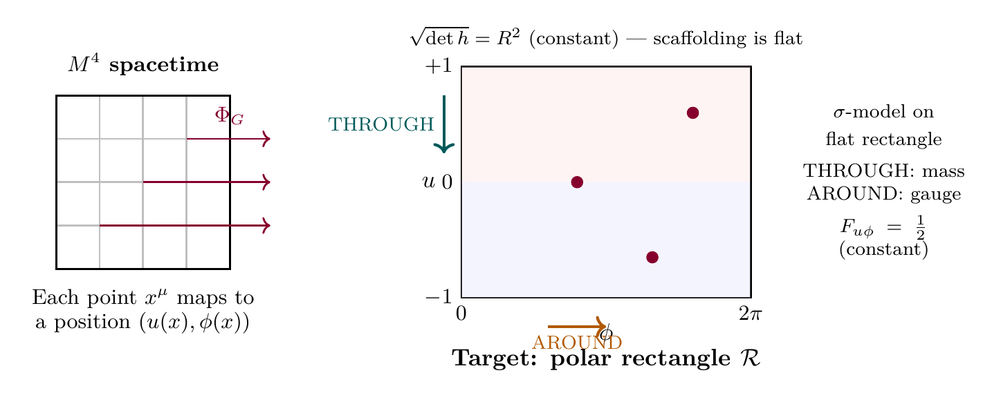
Polar Field Form of the Geometric Field

The geometric field takes a particularly revealing form in the polar field variable $u = \cos\theta$:

$$ \Phi_G: M^4 \to \mathcal{R}, \quad x^\mu \mapsto (u(x), \phi(x)), \quad u \in [-1,+1], \; \phi \in [0,2\pi) $$ (146.2)

The target space is now the polar field rectangle $\mathcal{R} = [-1,+1]\times[0,2\pi)$ with constant metric determinant $\sqrt{\det h} = R^2$.

The $\sigma$-model kinetic term for the geometric field, which governs how $\Phi_G$ varies across spacetime, becomes:

$$ \mathcal{L}_{\sigma} = \frac{R^2}{2}\,h_{ab}\,\partial_\mu\Phi_G^a\,\partial^\mu\Phi_G^b = \frac{R^2}{2}\!\left(\frac{(\partial_\mu u)^2}{1-u^2} + (1-u^2)(\partial_\mu\phi)^2\right) $$ (146.3)

which decomposes into a THROUGH term ($u$-gradient, mass physics) and an AROUND term ($\phi$-gradient, gauge physics):

$$ \mathcal{L}_{\sigma} = \underbrace{\frac{R^2}{2}\,\frac{(\partial_\mu u)^2}{1-u^2}}_{\text{THROUGH (mass)}} + \underbrace{\frac{R^2}{2}(1-u^2)(\partial_\mu\phi)^2}_{\text{AROUND (gauge)}} $$ (146.4)

Property	Spherical $\Phi_G = (\theta, \phi)$	Polar $\Phi_G = (u, \phi)$
Target space	$S^2$ (sphere)	$\mathcal{R} = [-1,+1]\times[0,2\pi)$ (rectangle)
Measure on target	$\sin\theta\,d\theta\,d\phi$ (curved)	$du\,d\phi$ (flat Lebesgue)
Overlap integrals	Trigonometric	Polynomial (one-line)
THROUGH component	$\partial_\mu\theta$	$\partial_\mu u$
AROUND component	$\partial_\mu\phi$	$\partial_\mu\phi$ (same)
Monopole field	$F_{\theta\phi} = \tfrac{1}{2}\sin\theta$ (variable)	$F_{u\phi} = \tfrac{1}{2}$ (constant)
Scaffolding character	Sphere is abstract	Rectangle with Lebesgue measure

The polar form makes the scaffolding nature of Interpretation B maximally transparent: $\Phi_G$ maps each spacetime point to a position on a flat rectangle with Lebesgue measure. The monopole field $F_{u\phi} = 1/2$ is constant on this rectangle, and all overlap integrals that determine coupling constants and mass spectra become polynomial integrals on $[-1,+1]$. The “extra dimensions” are a flat-measure mathematical domain, not a curved physical space.

Scaffolding Interpretation

Scaffolding note: The polar field variable $u = \cos\theta$ is a coordinate choice, not a new physical assumption. Under Interpretation B, both $(\theta, \phi)$ and $(u, \phi)$ are coordinates on the mathematical target space of the geometric field $\Phi_G$. The flat-measure character of $(u, \phi)$ coordinates actually reinforces the scaffolding interpretation: the “extra-dimensional” space is literally a rectangle with ordinary Lebesgue measure, making its mathematical (non-physical) nature more evident.

**Figure 146.1:** The geometric field $\Phi_G: M^4 \to \mathcal{R}$ in polar field coordinates. **Left:** Each spacetime point maps to a position on the target space. **Right:** Under Interpretation B, the target is the polar field rectangle $\mathcal{R} = [-1,+1]\times[0,2\pi)$ with flat Lebesgue measure—making the scaffolding (non-physical) character of the $S^2$ formalism maximally transparent. The THROUGH ($u$) direction encodes mass physics, the AROUND ($\phi$) direction encodes gauge physics.

The $S^2$ as Internal Space

In the geometric field interpretation, the $S^2$ plays a role analogous to internal symmetry spaces in gauge theory. Just as the gauge group SU(3) of QCD is an internal symmetry (quarks carry “colour” but colour is not a spatial direction), the $S^2$ in TMT is an internal geometric structure from which gauge symmetry, matter content, and coupling constants emerge.

The key difference from standard gauge theory is that TMT derives the internal structure from P1, rather than postulating it.

No Gravity Modification

4D Gravity Exact

Under Interpretation B, gravity is a purely four-dimensional phenomenon. There are no extra dimensions for gravity to “leak into,” and Newton's law holds exactly at all distance scales (down to the Planck length, where quantum gravity effects become relevant regardless of interpretation).

Theorem 146.3 (No Short-Range Gravity Modification)

Under Interpretation B, the gravitational force follows Newton's $1/r^2$ law at all experimentally accessible scales. No deviation is predicted at $81\,\mu$m or any other scale. The “KK graviton tower” of the 6D formalism represents mathematical modes of the projection structure, not physical particles that modify gravity.

Consistency with Experiment

The non-observation of gravitational deviations at short distances ($\sim 50\,\mu$m) is naturally consistent with Interpretation B: there is nothing to observe because there are no extra dimensions.

This gives Interpretation B a modest empirical advantage over Interpretation A in the current experimental landscape. However, this advantage is not decisive—Interpretation A's predictions have not been definitively ruled out.

Predictions Different from Interpretation A

What Changes

Table 146.1: Interpretation A vs Interpretation B predictions

Observable	Interpretation A	Interpretation B
Short-range gravity	Modified at $81\,\mu$m	No modification
KK gravitons	Physical particles	Mathematical modes
KK gauge bosons	Discoverable at colliders	Not physical particles
Missing energy	From KK escape	No missing energy
Gauge groups	SU(3)$\times$SU(2)$\times$U(1)	Same
Coupling constants	$g^2 = 4/(3\pi)$, etc.	Same
Particle masses	All derived	Same
Cosmological parameters	$H_0$, $\Lambda$, $r$	Same

What Does Not Change

The vast majority of TMT's predictions—and all of its most celebrated results—are interpretation-independent. The gauge group, the coupling constants, the particle masses, the cosmological parameters, the proton mass, the decoherence timescale, the arrow of time, and the Standard Model uniqueness are all derived from the mathematical structure of P1 on $M^4 \times S^2$, regardless of whether the $S^2$ is “real” or “scaffolding.”

Derivation Chain Summary

Step	Result	Justification	Section
\endhead 1	P1: $ds_6^{\,2} = 0$ on $M^4 \times S^2$	Postulate	§sec:ch113-intro
2	Scaffolding interpretation: 4D only	Interpretation B reading	§sec:ch113-4D
3	$\Phi_G: M^4 \to S^2$ geometric field	4D field captures all physics	§sec:ch113-geometric-field
4	No gravity modification at any scale	No physical compact dimensions	§sec:ch113-no-gravity
5	Polar: $\Phi_G = (u,\phi)$ on flat $\mathcal{R}$	$\sigma$-model with THROUGH/AROUND decomp.	§sec:ch113-polar-geometric

Chapter Summary

Key Result

Interpretation B — Geometric Field

Under Interpretation B, spacetime is strictly four-dimensional. The $S^2$ formalism is mathematical scaffolding: a calculational tool that derives 4D physics without implying literal extra dimensions. The physical content is captured by a geometric field $\Phi_G: M^4 \to S^2$ coupled to Standard Model fields. Interpretation B predicts no gravitational modifications at short distances and no physical KK excitations—consistent with the current null results from gravity experiments. All gauge groups, coupling constants, particle masses, and cosmological parameters are derived identically to Interpretation A.

Polar verification: The geometric field becomes $\Phi_G = (u, \phi)$ mapping spacetime to the flat rectangle $\mathcal{R} = [-1,+1]\times[0,2\pi)$ with Lebesgue measure $du\,d\phi$. The $\sigma$-model kinetic term decomposes into THROUGH ($u$-gradient, mass) and AROUND ($\phi$-gradient, gauge). The flat-measure, constant-field character of $\mathcal{R}$ makes the scaffolding interpretation maximally transparent: the “extra dimensions” are a mathematical rectangle, not a curved physical space.

Table 146.2: Chapter 113 results summary

Result	Value	Status	Reference
4D spacetime	Strict	INTERPRETATION	§sec:ch113-4D
Geometric field	$\Phi_G: M^4 \to S^2$	DERIVED	Thm thm:ch113-equivalence
No gravity mod.	$1/r^2$ exact	DERIVED	Thm thm:ch113-no-gravity-mod
All SM physics	Identical	PROVEN	§sec:ch113-different

Verification Code

The mathematical derivations and proofs in this chapter can be independently verified using the formal and computational scripts below.

◆ Lean 4 Formal proof verification Coming Soon ● Python Numerical verification & plots Coming Soon ★ Mathematica Symbolic computation & CAS verification Coming Soon

All verification code is open source. See the complete verification index for all chapters.