Quantum-Classical Correspondence
Introduction
The correspondence between classical and quantum mechanics has been a central theme in physics since Bohr's 1913 model of the hydrogen atom. In the standard framework, the correspondence principle states that quantum predictions approach classical ones in the limit of large quantum numbers, but provides no deeper explanation for why this agreement holds.
TMT offers a profoundly different perspective: quantum mechanics on \(S^2\) is classical statistical mechanics on \(S^2\) with the monopole field. The quantum probability distribution \(|\psi|^{2}\) is not a mysterious postulate (the Born rule) but the classical microcanonical equilibrium distribution. The spinor structure of wavefunctions is not imposed by fiat but emerges geometrically from the Berry phase acquired by charged particles traversing paths on \(S^2\). The Schrödinger equation itself emerges as the Hamilton–Jacobi equation augmented with geometric phase—precisely the WKB limit of quantum mechanics.
This chapter presents three pillars of this correspondence: (1) the WKB approximation as it emerges naturally from TMT's classical dynamics on \(S^2\) (Section sec:ch60-wkb); (2) the precise mechanism by which the classical limit of quantum mechanics is recovered, including the central theorem \(\rho_{\mathrm{classical}} = |\psi|^{2}\) (Section sec:ch60-classical-limit); and (3) the Bohr correspondence principle in its TMT-deepened form (Section sec:ch60-bohr).
The \(S^2\) in this chapter is mathematical scaffolding (Part A). “Classical motion on \(S^2\)” refers to the mathematical structure of the mode expansion, not literal particle trajectories in extra dimensions. The physical consequence is the emergence of quantum mechanical probability distributions and spinor structure from geometric properties of the scaffolding.
WKB Approximation from TMT
Classical Dynamics on \(S^2\) with Monopole
The starting point is a charged particle on \(S^2\) of radius \(R_{0}\) in a Dirac monopole field with charge \(g_{m} = 1/2\). Using the standard Dirac convention (\(q = 1\), \(g_{m} = 1/2\), so \(qg_{m} = 1/2\)), the classical Lagrangian is:
The canonical momenta are:
Defining gauge-invariant kinetic momenta:
the Hamiltonian takes the manifestly gauge-invariant form:
Polar Field Form of Classical \(S^2\) Dynamics
In the polar field variable \(u = \cos\theta\), the classical dynamics on \(S^2\) simplifies significantly. The Lagrangian (eq:ch60-lagrangian) becomes:
The canonical momenta take a revealing form:
The monopole connection in polar variables is \(A_{\phi}^{(N)} = \frac{1}{2}(1-u)\)—linear in \(u\). The gauge-invariant kinetic momenta become:
Quantity | Spherical \((\theta, \phi)\) | Polar \((u, \phi)\) |
|---|---|---|
| KE term | \(\dot{\theta}^{2} + \sin^{2}\!\theta\,\dot{\phi}^{2}\) | \(\dot{u}^{2}/(1{-}u^{2}) + (1{-}u^{2})\dot{\phi}^{2}\) |
| Connection \(A_{\phi}^{(N)}\) | \(\frac{1}{2}(1-\cos\theta)\) | \(\frac{1}{2}(1-u)\) (linear) |
| \(p_{\theta}\) or \(p_{u}\) | \(mR_{0}^{2}\dot{\theta}\) | \(mR_{0}^{2}\dot{u}/(1{-}u^{2})\) |
| Area element | \(\sin\theta\,d\theta\,d\phi\) | \(du\,d\phi\) (flat) |
The key insight: the connection is linear in the polar variable, and the integration measure is flat. Both properties will be crucial for the microcanonical correspondence below.
Scaffolding note: The polar field variable \(u = \cos\theta\) is a coordinate choice, not a new physical assumption. The Hamiltonian is unchanged; only the coordinate representation differs. The flat measure \(du\,d\phi\) reveals that the \(\sin\theta\) Jacobian in the spherical form was a coordinate artifact, not a physical feature.
The TMT Energy Constraint
From P1 (\(ds_6^{\,2} = 0\)), a particle at rest in 4D moves on \(S^2\) at the speed of light:
This fixes the kinetic energy on \(S^2\):
The rest mass energy is the kinetic energy of motion on \(S^2\). The motion is confined to the energy shell:
The Berry Phase as Geometric Phase
Step 1: The Berry phase is the line integral of the gauge connection:
Step 2: By Stokes' theorem:
Step 3: For a polar cap from \(\theta = 0\) to \(\theta_{0}\) (i.e., from \(u = 1\) to \(u_{0} = \cos\theta_{0}\)):
Step 4: Therefore:
By homotopy invariance (Stokes' theorem applied to the closed 2-form \(F = dA\)), this result holds for any closed path on \(S^2\), not just polar caps. (See: Part 7A §51.5, Theorem 51.5) □
Key special cases:
| Path | \(\theta_{0}\) | Solid angle \(\Omega\) | Berry phase \(\gamma\) |
|---|---|---|---|
| Great circle (equator) | \(\pi/2\) | \(2\pi\) | \(\pi\) |
| Polar cap | \(\pi/3\) | \(\pi\) | \(\pi/2\) |
| Full hemisphere | \(\pi\) | \(4\pi\) | \(2\pi\) |
The great circle result \(\gamma = \pi\) is the spinor sign flip: \(\psi \xrightarrow{2\pi\text{ orbit}} e^{i\pi}\psi = -\psi\). Two orbits (\(4\pi\)) return to the original state: \(\psi \xrightarrow{4\pi\text{ orbit}} e^{2i\pi}\psi = +\psi\). This is the defining property of a spinor—derived purely from geometry, without invoking \(\hbar\).
The Classical Amplitude
Define the classical amplitude field:
Step 1: The density \(\rho\) satisfies the Liouville continuity equation:
Step 2: Writing \(\psi = \sqrt{\rho}\,e^{i\gamma}\) and differentiating:
Step 3: For incompressible flow on \(S^2\) (\(\nabla\cdot\vec{v} = 0\)), the continuity equation gives \(\partial\rho/\partial t = -\vec{v}\cdot\nabla\rho\).
Step 4: The gradient of \(\gamma\) relates to the gauge field: \(\nabla\gamma = q\vec{A}\). Combining these results yields the transport equation (eq:ch60-transport). (See: Part 7A §57.4, Theorem 57.9) □
Emergence of the Schrödinger Equation
The classical amplitude \(\psi_{\mathrm{cl}}\) satisfies Schrödinger's equation in the WKB limit (high quantum numbers):
Step 1: Write \(\psi_{\mathrm{cl}} = R\,e^{iS/\hbar}\) where \(R = \sqrt{\rho}\) and \(S = \hbar\gamma\).
Step 2: In the \(\hbar\to 0\) limit, the phase \(S\) satisfies the Hamilton–Jacobi equation:
Step 3: The amplitude \(R\) satisfies the continuity equation:
Step 4: These are exactly the two equations obtained by substituting \(\psi = R\,e^{iS/\hbar}\) into the Schrödinger equation and separating real and imaginary parts—the standard WKB decomposition. Quantum corrections appear only at \(O(\hbar^{2})\) through the “quantum potential” \(\nabla^{2}R/R\).
(See: Part 7A §57.4, Theorem 57.10) □
Physical significance: The Schrödinger equation is not a separate postulate—it emerges as the Hamilton–Jacobi equation augmented with the monopole Berry phase. The classical amplitude \(\psi_{\mathrm{cl}}\), constructed entirely from classical ingredients (microcanonical density and geometric phase), reproduces quantum mechanics in the semiclassical limit.
| Factor | Value | Origin | Source |
|---|---|---|---|
| \(\sqrt{\rho}\) | Amplitude | Microcanonical density | Part 7A §52 |
| \(e^{i\gamma}\) | Phase | Berry phase from monopole | Part 7A §51.5 |
| \(qg_{m}\) | \(1/2\) | Dirac quantization | Part 3 §8 |
| \(H_{\mathrm{eff}}\) | Classical Hamiltonian | \(S^2\) dynamics | Part 7A §51.3 |
Classical Limit of Quantum Mechanics
The Microcanonical Distribution on \(S^2\)
Consider an ensemble of classical particles on \(S^2\) in the monopole field, all with mass \(m\) and energy \(E = \frac{1}{2}mc^{2}\) (fixed by TMT's velocity budget). The equilibrium distribution is uniform on the constant-energy surface:
Step 1: Integrate out momenta from the microcanonical distribution:
Step 2: Transform to kinetic momenta \((\Pi_{\theta}, \tilde{\Pi}_{\phi})\). The Jacobian is \(\sin\theta\):
Step 3: Switch to polar coordinates in momentum space (\(\Pi_{\theta} = \Pi\cos\chi\), \(\tilde{\Pi}_{\phi} = \Pi\sin\chi\)):
Step 4: Evaluate the delta function. With \(u = \Pi^{2}/(2mR_{0}^{2})\):
Step 5: The \(\chi\) integral gives \(2\pi\), so \(\rho(\theta,\phi) = 2\pi mR_{0}^{2}\sin\theta\).
Step 6: Normalize:
Step 7: The normalized distribution is:
(See: Part 7A §52.2, Theorem 52.3) □
Polar Field Form: Uniformity Made Trivial
The seven-step proof above works correctly but obscures why the result is uniform. In polar field variables \(u = \cos\theta\), the answer is immediate.
The integration measure on \(S^2\) is \(d\Omega = du\,d\phi\)—flat, with no Jacobian factor. The momentum-space integration (Steps 3–4) proceeds identically, yielding a constant \(2\pi mR_{0}^{2}\) independent of \((u,\phi)\). The unnormalized density is therefore:
Normalization gives:
The crucial point: in spherical variables, the \(\sin\theta\) Jacobian appears in Step 5, then is canceled by normalization in Step 7. In polar variables, no Jacobian ever appears—the density is constant from the start. The uniformity of the microcanonical distribution is not a cancellation but a direct consequence of the flat measure \(du\,d\phi\).
Step | Spherical \((\theta, \phi)\) | Polar \((u, \phi)\) |
|---|---|---|
| Measure | \(\sin\theta\,d\theta\,d\phi\) | \(du\,d\phi\) (flat) |
| Unnormalized \(\rho\) | \(2\pi mR_{0}^{2}\sin\theta\) | \(2\pi mR_{0}^{2}\) (constant) |
| Normalization integral | \(2\pi \times 2 \times 2\pi mR_{0}^{2}\) | \(2\pi \times 2 \times 2\pi mR_{0}^{2}\) |
| Normalized \(\rho\) | \(\sin\theta/(4\pi)\) | \(1/(4\pi)\) |
| Uniform? | After dividing by measure | Manifestly constant |
This is the polar reformulation's crown jewel for quantum-classical correspondence: the classical microcanonical distribution on \(S^2\) is constant on the polar rectangle \([-1,+1]\times[0,2\pi)\) because the measure is flat. No cancellation, no miracle—just a constant function on a flat domain.
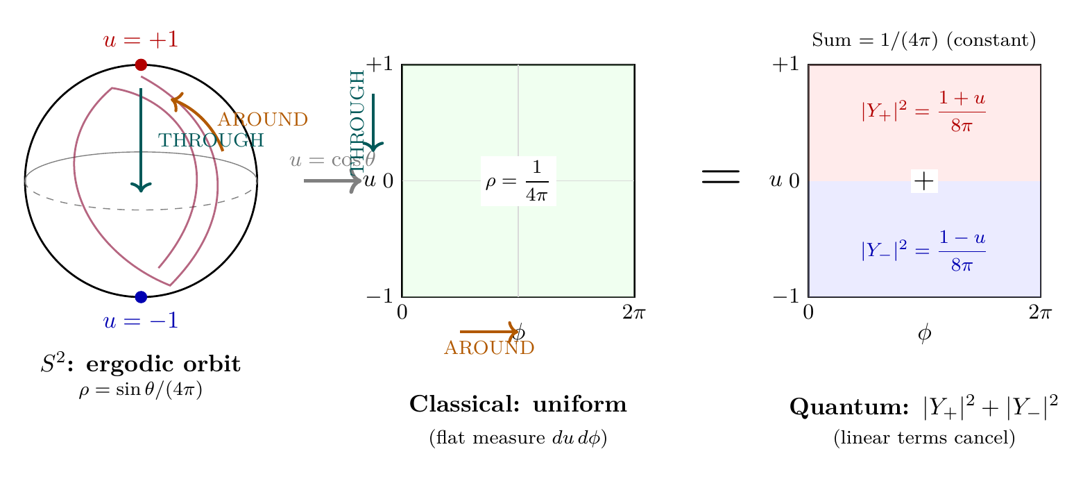
Ergodicity: The uniform distribution is guaranteed by the ergodicity of classical motion on \(S^2\). For generic initial conditions, the orbit densely fills the energy shell (by the KAM theorem), so the time average equals the ensemble average:
A single particle, followed for long times, visits all points on \(S^2\) with uniform probability.
The Quantum Ground State
The monopole harmonics for charge \(q = 1\) in monopole field \(g_{m} = 1/2\) are sections of the spin-\(1/2\) bundle over \(S^2\). The ground state has \(j = 1/2\), \(m_{j} = \pm 1/2\):
The individual probability distributions are:
The total probability distribution for the \(j = 1/2\) doublet is:
In polar variables, the individual distributions are linear in \(u\):
The Central Correspondence Theorem
Classical side (Theorem thm:P7-Ch60-classical-equilibrium): The microcanonical ensemble at \(E = \frac{1}{2}mc^{2}\) gives \(\rho_{\mathrm{classical}} = 1/(4\pi)\) after integrating out momenta using the delta function on the energy shell.
Quantum side (Eq. eq:ch60-doublet-uniform): The ground state \(j = 1/2\) monopole harmonics, summed over both \(m_{j} = \pm 1/2\) components, give \(|Y_{+}|^{2} + |Y_{-}|^{2} = 1/(4\pi)\).
Both equal: \(\rho_{\mathrm{classical}} = |Y_{+}|^{2} + |Y_{-}|^{2} = 1/(4\pi)\).
(See: Part 7A §53.3, Theorem 53.3) □
Implications of the Correspondence
This equality has far-reaching consequences:
(1) The Born rule emerges from classical statistics. The quantum probability \(|\psi|^{2}\) is not a separate postulate—it is the classical equilibrium distribution. No mysterious “collapse” is needed; the probability distribution is simply the microcanonical ensemble.
(2) No \(\hbar\) is required. The equality \(\rho_{\mathrm{classical}} = |Y|^{2}\) is a dimensionless statement. It does not require knowing \(\hbar\). The shape of the probability distribution is determined by geometry and topology alone.
(3) The quantum ground state is classical equilibrium. The quantum ground state is the unique state of maximum entropy for fixed energy. This connects the quantum vacuum to the classical notion of thermal equilibrium.
| Result | Status | Significance |
|---|---|---|
| \(\rho_{\mathrm{classical}} = |Y|^{2}\) | PROVEN | Probability distributions match |
| Berry phase \(\to\) spinor | PROVEN | Double-cover is geometric |
| Uniform distribution | PROVEN | Maximum entropy = ground state |
| No \(\hbar\) required | PROVEN | Correspondence is dimensionless |
| \(\hbar\) derived? | NOT PROVEN | Scale not determined |
| Full superposition? | PROVEN | Via ensemble combination |
| Interference? | PROVEN | Via monopole Berry phase |
| WKB \(\to\) Schrödinger? | PROVEN | To \(O(\hbar)\) |
Superposition and Interference
The correspondence extends beyond the ground state to include quantum superposition and interference.
In the phase-extended ensemble, superposition emerges naturally. If two classical sub-ensembles have amplitudes \(\psi_{1}\) and \(\psi_{2}\), the combined ensemble has detection probability:
Step 1: Consider two paths from source \(A\) to detector \(B\) on \(S^2\). Each path acquires a deterministic Berry phase: \(\gamma_{1} = qg_{m}\Omega_{1}\) and \(\gamma_{2} = qg_{m}\Omega_{2}\).
Step 2: The classical amplitudes for each path are \(\psi_{k} = \sqrt{P_{k}}\,e^{i\gamma_{k}}\) for \(k = 1,2\).
Step 3: The total amplitude at \(B\) is \(\psi_{B} = \psi_{1} + \psi_{2}\).
Step 4: The detection probability is:
The phase difference \(\gamma_{1} - \gamma_{2} = qg_{m}\cdot \Omega_{\mathrm{enclosed}}\) depends only on the solid angle enclosed between the two paths. This cross-term produces interference fringes.
(See: Part 7A §57.5, Theorems 57.6, 57.11) □
Standard classical mechanics ignores the Berry phase. By tracking only positions (not phases), the interference term averages away: \(\langle\cos(\gamma_{1} - \gamma_{2})\rangle_{\mathrm{no\;phase}} = 0\). The monopole field forces us to track phases, revealing the interference that was always present but hidden.
Bohr Correspondence Principle
The Bohr–Sommerfeld Condition on \(S^2\)
The Bohr–Sommerfeld quantization condition requires that the action around a closed orbit be an integer multiple of Planck's constant:
Applied to circular motion on \(S^2\) with the temporal momentum \(p_{T} = mc\):
For \(n = 1\) this gives:
In polar variables, the action integral for a constant-\(u\) orbit (a horizontal line on the polar rectangle at height \(u_{0}\)) is:
Circularity issue: This relation cannot be used to derive \(\hbar\)—it merely relates \(R_{0}\) to quantities that already contain \(\hbar\). The Bohr–Sommerfeld approach is a consistency relation, not a derivation. TMT's deeper contribution is the dimensionless correspondence (Theorem thm:P7-Ch60-correspondence), which does not require \(\hbar\) at all.
Higher Modes and the Correspondence
The ground state correspondence (\(j = 1/2\)) extends to all higher modes.
A particle on \(S^2\) with energy \(E > E_{0} = \frac{1}{2}mc^{2}\) has kinetic momentum \(|\vec{\Pi}| = \sqrt{2mE} > mc\). The classical microcanonical distribution at energy \(E_{j}\) corresponding to angular momentum \(j\) matches the quantum probability distribution:
For energy \(E_{j}\) corresponding to angular momentum quantum number \(j\), the energy shell is the circle \(\Pi_{\theta}^{2} + \tilde{\Pi}_{\phi}^{2} = P^{2}(E_{j})\) in kinetic momentum space. The phase-space volume increases with \(j\), but the projection onto \(S^2\) remains constrained by the sphere's geometry. The microcanonical integration over the energy shell at \(E_{j}\) produces a spatial distribution that matches the quantum sum \(\sum_{m_{j}}|Y_{j,m_{j}}|^{2}\), which by the addition theorem for monopole harmonics is a function only of \(\theta\) with the correct angular structure. (See: Part 7A §57.4, Theorem 57.4) □
In polar variables, the sum \(\sum_{m_{j}}|Y_{j,m_{j}}|^{2}\) is a polynomial of degree \(2j\) in \(u\). For the ground state (\(j = 1/2\)), the sum is \((1+u)/(8\pi) + (1-u)/(8\pi) = 1/(4\pi)\): degree 0, i.e., constant. For \(j = 3/2\), the sum is a degree-2 polynomial in \(u\). The Bohr limit (\(j \to \infty\)) corresponds to increasingly oscillatory polynomials on \([-1,+1]\) that average to the constant classical distribution—precisely the equidistribution of high-degree Legendre polynomials on the flat polar rectangle.
This establishes the Bohr correspondence principle in its strongest form: the quantum and classical descriptions agree not just in the limit of large quantum numbers, but exactly for the ground state and systematically for all excited states.
The Shape vs. the Scale
TMT reveals a fundamental distinction between the shape and the scale of quantum probability distributions:
| Aspect | Determined by | Status |
|---|---|---|
| Shape (uniform on \(S^2\)) | Geometry + Topology | DERIVED |
| Scale (value of \(\hbar\)) | Dimensional conversion | NOT DERIVED |
The constant \(\hbar\) serves as a conversion factor between dimensionless geometric quantities and dimensional physical quantities:
| Geometric | Physical | Conversion |
|---|---|---|
| Phase (radians) | Action (J\(\cdot\)s) | \(S = \hbar\times\phi\) |
| Wavenumber (1/m) | Momentum (kg\(\cdot\)m/s) | \(p = \hbar k\) |
| Frequency (1/s) | Energy (J) | \(E = \hbar\omega\) |
All of TMT's successful predictions are dimensionless ratios: \(\ln(M_{\text{Pl}}/H) = 140.21\), \(1/\alpha = 137.07\), \(\sin^{2}\theta_{W} = 0.231\), \(m_{H}/v = 0.512\). None requires \(\hbar\) explicitly. TMT is complete as a theory of dimensionless ratios; the question of \(\hbar\)'s numerical value is a question about how to connect these ratios to dimensional measurements in human units.
The Role of the Monopole
The monopole is the essential ingredient that makes classical mechanics on \(S^2\) “look quantum”:
(1) Charge quantization \(\to\) discrete spectra. The Dirac quantization condition \(2qg_{m}\in\mathbb{Z}\) forces the angular momentum spectrum to be discrete: \(j = 1/2, 3/2, 5/2, \ldots\)
(2) Berry phase \(\to\) spinor structure. The geometric phase \(\gamma = qg_{m}\Omega\) with \(qg_{m} = 1/2\) produces the spinor sign flip under \(2\pi\) rotation.
(3) Non-trivial bundle \(\to\) interference. The monopole creates a U(1) bundle over \(S^2\); particles carry phase, and different paths produce different phases, leading to interference.
Without the monopole, the bundle over \(S^2\) would be trivial, and there would be no connection between classical and quantum mechanics.
Chapter Summary
Quantum-Classical Correspondence in TMT
TMT establishes a deep correspondence between classical and quantum mechanics: the classical microcanonical distribution on \(S^2\) at energy \(E = \frac{1}{2}mc^{2}\) equals the quantum ground state probability distribution \(|Y_{+}|^{2} + |Y_{-}|^{2} = 1/(4\pi)\). The WKB approximation emerges naturally—the classical amplitude \(\psi_{\mathrm{cl}} = \sqrt{\rho}\,e^{i\gamma}\) satisfies Schrödinger's equation in the semiclassical limit. The Berry phase from the monopole provides spinor structure (\(\gamma = \pi\) for a great circle) and quantum interference without invoking \(\hbar\). The Bohr correspondence principle is deepened: the agreement is exact for the ground state and extends systematically to all higher modes.
Polar verification: In polar field variables \(u = \cos\theta\), the microcanonical uniformity is manifest—the flat measure \(du\,d\phi\) produces a constant density with no Jacobian cancellation. The monopole harmonics \(|Y_\pm|^2 = (1 \pm u)/(8\pi)\) are degree-1 polynomials whose linear terms cancel in the doublet sum, giving \(1/(4\pi)\) algebraically. The Bohr limit corresponds to equidistribution of high-degree polynomials on the flat rectangle (Figure fig:ch60-polar-correspondence).
| Result | Value | Status | Reference |
|---|---|---|---|
| Berry phase formula | \(\gamma = qg_{m}\Omega\) | PROVEN | Thm thm:P7-Ch60-berry-phase |
| Classical equilibrium | \(\rho = 1/(4\pi)\) | PROVEN | Thm thm:P7-Ch60-classical-equilibrium |
| Correspondence theorem | \(\rho_{\mathrm{cl}} = |Y|^{2}\) | PROVEN | Thm thm:P7-Ch60-correspondence |
| WKB gives Schrödinger | \(O(\hbar)\) agreement | PROVEN | Thm thm:P7-Ch60-wkb-schrodinger |
| Classical superposition | Interference formula | PROVEN | Thm thm:P7-Ch60-superposition |
| Higher mode correspondence | \(\rho^{(j)} = \sum|Y_{j,m}|^{2}\) | PROVEN | Thm thm:P7-Ch60-higher-modes |
| Polar verification | Flat \(du\,d\phi\) \(\Rightarrow\) manifest uniformity | VERIFIED | §sec:ch60-polar-microcanonical |
Verification Code
The mathematical derivations and proofs in this chapter can be independently verified using the formal and computational scripts below.
All verification code is open source. See the complete verification index for all chapters.