Chapter 52

Gravity in TMT

Introduction

With the fermion mass sector complete (Part VII), we now turn to gravity. In the Standard Model, gravity is not included at all—the three gauge forces (electromagnetic, strong, and weak) are described by quantum field theory, while gravity is described separately by general relativity. Unifying these descriptions is one of the deepest open problems in physics.

TMT provides a fundamentally different perspective on gravity. Rather than treating gravity as a fourth force to be unified with the other three, TMT derives gravity as the conservation-enforcement mechanism for temporal momentum across the $S^2$ scaffolding structure. The key insight is that P1 ($ds_6^{\,2} = 0$) forces the scaffolding stress-energy tensor to be traceless, and this tracelessness condition, when decomposed into 4D and $S^2$ contributions, produces the statement that gravity couples to temporal momentum density—what we observe as rest mass.

This chapter establishes three central results:

(1) The scalar gravitational field couples to temporal momentum density $\rho_{p_T} = \rho_0 c$, not to energy density (P3, derived from P1).

(2) Gravity is not a fundamental force in the same category as the gauge forces—it is the interface response mechanism of the $S^2$ scaffolding.

(3) The gravitational coupling is conservation-driven: it enforces the balance between 4D and $S^2$ contributions required by tesseract conservation.

Scaffolding Interpretation

The derivations in this chapter use the $M^4 \times S^2$ scaffolding formalism. Per Part A, the 6D structure is mathematical scaffolding encoding 4D physics, not literal extra dimensions. The physical content is that gravity couples to temporal momentum (rest mass), not energy. All predictions are 4D observables.

Coupling to Temporal Momentum

The Tracelessness Theorem

The foundation of TMT's gravitational theory is a single, powerful consequence of P1.

Theorem 52.1 (Scaffolding Tracelessness)

The scaffolding stress-energy tensor is traceless:

$$ T^A_A = 0 $$ (52.1)

where $A$ runs over all six scaffolding indices ($\mu = 0,1,2,3$ for $M^4$ and $i = 4,5$ for $S^2$).

Proof.

Step 1: P1 states $ds_6^{\,2} = 0$ for massive particles. In momentum-space, this becomes the null constraint:

$$ k^A k_A = 0 $$ (52.2)

where $k^A$ is the scaffolding 6-momentum.

Step 2: The scaffolding 6-velocity $u^A = k^A/m$ inherits the null property:

$$ u^A u_A = 0 $$ (52.3)

Step 3: For dust (pressureless matter), the scaffolding stress-energy tensor is:

$$ T^{AB} = \rho \, u^A u^B $$ (52.4)

Step 4: Taking the trace:

$$ T^A_A = g_{AB} T^{AB} = \rho \, g_{AB} u^A u^B = \rho \, u^A u_A = \rho \cdot 0 = 0 $$ (52.5)

The trace vanishes identically as a consequence of the null constraint. (See: Part 1 §3.1, Theorem 3.1) □

Decomposition into 4D and $S^2$ Contributions

The tracelessness condition connects 4D physics to the $S^2$ scaffolding structure.

The scaffolding trace decomposes as:

$$ T^A_A = T^\mu_\mu + T^i_i = 0 $$ (52.6)

where $T^\mu_\mu$ is the 4D trace and $T^i_i$ is the $S^2$ trace.

This decomposition has a profound physical consequence: the 4D and $S^2$ contributions must exactly balance. Defining:

$$\begin{aligned} T_4 &\equiv T^\mu_\mu \quad\text{(4D trace)} \\ T_{S^2} &\equiv T^i_i \quad\text{($S^2$ trace)} \end{aligned}$$ (52.29)

the tracelessness condition becomes:

$$ T_4 + T_{S^2} = 0 \quad\Rightarrow\quad T_4 = -T_{S^2} $$ (52.7)

For a massive particle at rest, the 4D trace is:

$$ T^\mu_\mu = -\rho_0 c^2 $$ (52.8)

while the $S^2$ trace is:

$$ T^i_i = +\rho_0 c^2 $$ (52.9)

The balance is exact: the rest mass energy density in 4D is precisely compensated by the $S^2$ contribution. This balance is tesseract conservation.

Polar Field Form of the Trace Balance

The $S^2$ trace $T_{S^2} = T^i_i$ acquires a transparent physical decomposition in the polar field variable $u = \cos\theta$:

$$ T_{S^2} = T^u{}_u + T^\phi{}_\phi $$ (52.10)

where $T^u{}_u$ is the THROUGH (polar, mass) stress and $T^\phi{}_\phi$ is the AROUND (azimuthal, gauge) stress.

The tesseract conservation condition becomes:

$$ T_4 + T^u{}_u + T^\phi{}_\phi = 0 $$ (52.11)

Property	Spherical $(\theta, \phi)$	Polar $(u, \phi)$
$S^2$ trace	$T^\theta{}_\theta + T^\phi{}_\phi$	$T^u{}_u + T^\phi{}_\phi$
THROUGH stress	$\rho R^2 \dot\theta^2$	$\rho R^2 \dot{u}^2/(1-u^2)$
AROUND stress	$\rho R^2 \sin^2\!\theta\,\dot\phi^2$	$\rho R^2 (1-u^2)\dot\phi^2$
Metric determinant	$R^4 \sin^2\!\theta$ (variable)	$R^4$ (constant)
Physical interpretation	Mixed Jacobian factors	Clean: THROUGH $+$ AROUND

The key insight: in polar coordinates, the three-channel balance eq:ch51-three-channel-balance directly exhibits how gravity (which couples to the total $T_4 = -T_{S^2}$) sees the sum of both $S^2$ channels, while gauge forces act within individual channels.

Scaffolding Interpretation

Scaffolding note: The polar field variable $u = \cos\theta$ is a coordinate choice, not a new physical assumption. The THROUGH/AROUND decomposition of $T_{S^2}$ is coordinate-independent, but its clean separation into $T^u{}_u$ and $T^\phi{}_\phi$ with constant metric determinant $\sqrt{\det h} = R^2$ is a computational advantage of the polar representation.

Why Gravity Couples to the Trace

The gravitational field in TMT includes, in addition to the tensor graviton of general relativity, a scalar component $\Phi$ arising from fluctuations of the $S^2$ modulus (the characteristic geometric relationship scale $R$).

The scalar field $\Phi$ is a Lorentz scalar (gauge-invariant, real). Therefore it can only couple to a Lorentz-invariant source. The only Lorentz scalar that can be constructed from the stress-energy tensor $T_{\mu\nu}$ is its trace:

$$ \mathcal{L}_{\mathrm{int}} = -\frac{\Phi}{2M_{\text{Pl}}} \, T^\mu_\mu $$ (52.12)

Since $T^\mu_\mu = -\rho_0 c^2 = -\rho_{p_T} \cdot c$, this coupling is precisely to temporal momentum density.

The Complete Derivation Chain

The coupling of gravity to temporal momentum follows from a 15-step derivation chain, each step proven from P1:

Theorem 52.2 (P3: Gravity Couples to Temporal Momentum)

The scalar gravitational field couples to temporal momentum density:

$$ \boxed{\rho_{\mathrm{grav}} = \rho_{p_T} = \rho_0 c} $$ (52.13)

Equivalently, the scalar gravity–matter interaction Lagrangian is:

$$ \mathcal{L}_{\mathrm{int}} = -\frac{\Phi}{2M_{\text{Pl}}} \, T^\mu_\mu = +\frac{\Phi}{2M_{\text{Pl}}} \, \rho_{p_T} \cdot c $$ (52.14)

where $\Phi$ is the modulus scalar field and $M_{\text{Pl}}$ is the Planck mass.

Proof.

The complete chain from P1 to P3 proceeds through 15 steps:

Step 1: The metric $g_{AB}$ has monopole charge $q = 0$ (gauge-invariant, real tensor).

Step 2: $q = 0$ implies volume integration over $S^2$ is valid for the gravitational action (the graviton goes THROUGH the $S^2$ surface, not AROUND it).

Step 3: The scaffolding gravitational action is:

$$ S = \frac{M_*^4}{2} \int d^4x \, d^2\Omega \, \sqrt{-g_6} \, R_6 $$ (52.15)

where $M_*$ is the fundamental mass scale and $R_6$ is the scaffolding Ricci scalar.

Step 4: The volume element factorizes: $\sqrt{-g_6} = \sqrt{-g_4} \cdot R^2 \sin\theta$. In polar coordinates ($u = \cos\theta$), the $\sin\theta$ is absorbed into the measure change $d\theta \to du$, so $\sqrt{-g_6}\,d\theta\,d\phi = \sqrt{-g_4} \cdot R^2\,du\,d\phi$ with constant coefficient $R^2$—no angular-dependent Jacobian artifacts.

Step 5: Integration over $S^2$ gives: $\int d\Omega = \int_0^{2\pi}d\phi\int_{-1}^{+1}du = 4\pi$. The flat measure $du\,d\phi$ makes the $q = 0$ volume integration a trivial polynomial integral.

Step 6: The Ricci scalar decomposes: $R_6 = R_4 + 2/R^2 - \ldots$ (plus terms involving modulus gradients).

Step 7: The Kaluza–Klein relation emerges:

$$ M_{\text{Pl}}^2 = 4\pi R_0^2 M_*^4 $$ (52.16)

Step 8: Define the modulus scalar field: $\Phi = M_{\text{Pl}} \sigma$ where $R = R_0(1 + \sigma)$.

Step 9: Particle masses scale as $m \propto M_* \propto R^{-1/2}$, so the mass coupling exponent is $\beta = 1/2$.

Step 10: Mass variation under modulus fluctuation:

$$ \frac{\delta m}{m} = -\frac{\Phi}{2M_{\text{Pl}}} $$ (52.17)

Step 11: Matter Lagrangian variation: $\delta\mathcal{L}_m = \rho c^2 \Phi/(2M_{\text{Pl}})$.

Step 12: The stress-energy trace: $T^\mu_\mu = -\rho_0 c^2$.

Step 13: The interaction Lagrangian: $\mathcal{L}_{\mathrm{int}} = -\Phi T^\mu_\mu / (2M_{\text{Pl}})$.

Step 14: Connection to temporal momentum:

$$ T^\mu_\mu = -\rho_0 c^2 = -\rho_{p_T} \cdot c $$ (52.18)

since $\rho_{p_T} = \rho_0 c$ is the temporal momentum density.

Step 15: Therefore gravity couples to temporal momentum density, which is what we observe as rest mass density. $\blacksquare$

(See: Part 1 §3.3A, Theorems 3.A2–3.A13, Theorem 3.5) □

Table 52.1: Factor Origin Table for the gravity–temporal momentum coupling

Factor	Value	Origin	Source
$q = 0$	Gravity monopole charge	Metric is real, gauge-invariant	Part 1 Thm 3.A2
$4\pi$	$S^2$ solid angle	$\int d\Omega = 4\pi$	Part 1 Thm 3.A5
$\beta = 1/2$	Mass–modulus coupling	$m \propto R^{-1/2}$	Part 1 Thm 3.A9
$M_{\text{Pl}}$	Planck mass	KK relation $M_{\text{Pl}}^2 = 4\pi R_0^2 M_*^4$	Part 1 Thm 3.A7
$-\rho_0 c^2$	4D trace value	Dust stress-energy trace	Part 1 Thm 3.A11

Physical Consequences of P3

The coupling of gravity to temporal momentum (rest mass) rather than energy has several profound consequences:

(1) Hot gas and cold gas gravitate the same. The rest mass content is identical regardless of temperature, so the scalar gravitational source is the same.

(2) Photons do not source scalar gravity. Photons have energy but zero rest mass, so $\rho_{p_T} = 0$ for radiation. (Photons still respond to tensor gravity—they follow geodesics of the full metric.)

(3) Relativistic particles gravitate less than naively expected. Their $T_{00} = \gamma^2 \rho_0 c^2$ is large, but $T^\mu_\mu = -\rho_0 c^2$ is velocity-independent.

(4) Vacuum energy does not gravitate. The vacuum has $\langle\rho_0\rangle = 0$, so $\langle T^\mu_\mu\rangle = 0$. This is how TMT addresses the cosmological constant problem: quantum vacuum fluctuations have enormous energy density but zero rest mass density, so they do not source scalar gravity.

Table 52.2: TMT vs General Relativity: gravitational sources

Source	GR	TMT (scalar sector)
Dust at rest	$\rho c^2$	$\rho_0 c^2 = \rho_{p_T} \cdot c$
Moving dust	$\gamma^2 \rho_0 c^2$ (increases)	$\rho_0 c^2$ (unchanged)
Hot matter ($\gamma \gg 1$)	Gravitates MORE	Gravitates SAME
Radiation	Sources gravity	Does NOT source $\Phi$
Vacuum ($\langle\rho_0\rangle = 0$)	May gravitate	Does NOT gravitate

Temporal Momentum Density Is Lorentz Invariant

A crucial property of temporal momentum density is its Lorentz invariance. For a particle with rest mass $m_0$:

$$ p_T = \frac{m_0 c}{\gamma} $$ (52.19)

The temporal momentum density involves the particle number density $n = \gamma n_0$ (Lorentz-contracted volume):

$$ \rho_{p_T} = n \cdot p_T = (\gamma n_0) \cdot \frac{m_0 c}{\gamma} = n_0 m_0 c = \rho_0 c $$ (52.20)

The $\gamma$ factors cancel exactly: the boost-induced increase in number density precisely compensates the decrease in individual temporal momentum. This cancellation is not accidental—it is a direct consequence of the Lorentz invariance of the trace $T^\mu_\mu$.

Contrast with energy density:

$$ \rho_E = \gamma^2 \rho_0 c^2 \quad\text{(frame-dependent)} $$ (52.21)

The Lorentz invariance of $\rho_{p_T}$ explains why the scalar gravitational coupling is frame-independent: the scalar field $\Phi$ is a Lorentz scalar, so it must couple to a Lorentz-invariant source. Temporal momentum density is precisely such a quantity.

Not a Fundamental Force

Gravity vs the Gauge Forces

In the Standard Model, the electromagnetic, strong, and weak forces are all gauge forces: they arise from local symmetries of the Lagrangian, are mediated by spin-1 gauge bosons, and act on particles carrying the corresponding charges (electric charge, color, weak isospin).

Gravity is fundamentally different. In TMT, this difference is explained: gravity is not a gauge force living on the $S^2$ scaffolding—it is the response of the scaffolding interface itself.

Table 52.3: Gravity vs gauge forces in TMT

Property	EM	Strong	Weak	Gravity
Acts on	Charge	Color	Weak isospin	All mass
Carrier	Photon	Gluon	$W^\pm, Z$	Spacetime
In SM	Gauge field	Gauge field	Gauge field	Not included
In TMT	Lives on $S^2$	Lives in $\mathbb{R}^3$	Lives on $S^2$	IS the interface
Monopole charge	$q \neq 0$	$q \neq 0$	$q \neq 0$	$q = 0$
Reduction method	Interface	Confinement	Interface	Volume

The Monopole Charge Distinction

The technical distinction between gravity and the gauge forces in TMT is cleanly captured by monopole charge.

Theorem 52.3 (Gravity Has Zero Monopole Charge)

The metric $g_{AB}$ has monopole charge $q = 0$.

Proof.

Step 1: The monopole on $S^2$ defines a U(1) gauge symmetry. Fields transform as $\Psi \to e^{iq\Lambda}\Psi$ under this U(1), where $q$ is the monopole charge.

Step 2: The metric $g_{AB}$ is a real, symmetric rank-2 tensor. Under any gauge transformation:

$$ g_{AB} \to g_{AB} $$ (52.22)

The metric is gauge-invariant because it measures distances—real quantities that cannot be multiplied by complex phases.

Step 3: Since $g_{AB} \to e^{i \cdot 0 \cdot \Lambda} g_{AB} = g_{AB}$:

$$ \boxed{q_{\mathrm{gravity}} = 0} $$ (52.23)

(See: Part 1 §3.3A.4, Theorem 3.A2) □

The consequence is immediate: fields with $q = 0$ go THROUGH the $S^2$ surface (volume integration valid), while fields with $q \neq 0$ go AROUND the $S^2$ surface (interface physics applies).

Table 52.4: Monopole charge determines dimensional reduction method

Field	Monopole charge	Reduction method
Scalar (uncharged)	$q = 0$	Volume integration (THROUGH)
Graviton (metric)	$q = 0$	Volume integration (THROUGH)
Charged fermion	$q \neq 0$	Interface physics (AROUND)
Gauge boson	$q \neq 0$	Interface physics (AROUND)

This is why gravity and the gauge forces have such different properties: they emerge from completely different mechanisms on the $S^2$ scaffolding. Gauge forces arise from the isometry group of $S^2$ acting on fields confined to the interface. Gravity arises from modulus fluctuations of the $S^2$ geometry itself, which propagate through the full volume.

Polar Field Form of the Gravity–Gauge Distinction

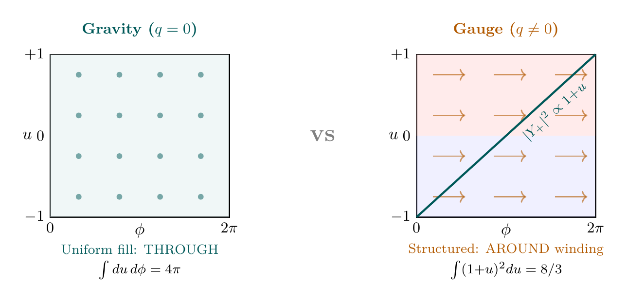
The monopole charge distinction becomes geometrically literal on the polar field rectangle $[-1,+1] \times [0,2\pi)$.

For gravity ($q = 0$): the gravitational action involves volume integration over $S^2$ with flat measure $du\,d\phi$:

$$ S_{\mathrm{grav}} \supset \int d^4x \int_{-1}^{+1} du \int_0^{2\pi} d\phi \; R^2 \sqrt{-g_4} \; \mathcal{L}_{\mathrm{grav}} $$ (52.24)

The integrand is polynomial in $u$ with constant measure—no $\sin\theta$ factors, no coordinate singularities in the integral. The graviton “fills” the polar rectangle uniformly.

For gauge fields ($q \neq 0$): the monopole harmonics $Y_\pm \propto (1 \pm u)^{1/2} e^{\pm i\phi/2}$ carry nontrivial $\phi$-dependence. The gauge coupling involves overlap integrals of the form:

$$ g^2 \propto \int_{-1}^{+1} (1+u)^2\,du \times \frac{1}{2\pi}\int_0^{2\pi} e^{i(q_1 - q_2)\phi}\,d\phi $$ (52.25)

The AROUND integral ($\phi$) enforces charge conservation via Kronecker delta $\delta_{q_1, q_2}$; the THROUGH integral ($u$) produces the polynomial factor that gives $g^2 = 4/(3\pi)$.

Property	Gravity ($q = 0$)	Gauge ($q \neq 0$)
Polar rectangle role	Uniform fill (volume)	Localized winding (interface)
$u$-dependence	None (constant)	Polynomial $(1 \pm u)^n$
$\phi$-dependence	None (azimuthally symmetric)	$e^{iq\phi}$ (winding)
Integration measure	$du\,d\phi$ (flat, trivial)	$du\,d\phi$ (flat, but integrand structured)
Channel	THROUGH (total $S^2$)	Individual AROUND / THROUGH
Physical mechanism	Modulus fluctuation	Isometry group action

The polar representation makes the gravity–gauge dichotomy visually obvious: gravity is the uniform background (constant on the rectangle), while gauge physics is the structured foreground (polynomial $\times$ winding modes on the rectangle).

**Figure 52.1:** Gravity vs gauge forces on the polar field rectangle. **Left:** Gravity ($q = 0$) fills the rectangle uniformly—the graviton has no $u$-dependence or $\phi$-winding, so volume integration with flat measure $du\,d\phi$ is trivial (THROUGH the entire $S^2$). **Right:** Gauge fields ($q \neq 0$) carry structured content: $\phi$-winding (orange AROUND arrows) and $u$-dependent monopole harmonic profiles (teal diagonal). The gauge coupling $g^2 = 4/(3\pi)$ emerges from the overlap integral of these structured modes.

Why Gravity Affects Time

In TMT, the connection between gravity and time is not mysterious. Gravity IS the response of the scaffolding interface, and temporal momentum is literally momentum in the temporal structure that constitutes mass.

The modulus scalar $\Phi$ represents fluctuations in the $S^2$ geometric relationship. When $\Phi$ varies in space, particle masses vary (since $m \propto R^{-1/2}$), and this mass variation manifests as a gravitational potential:

$$ V(r) = -\frac{GMm}{r} $$ (52.26)

The factor $m$ appearing here is the rest mass—temporal momentum divided by $c$. Gravity acts on temporal momentum because it is the mechanism that enforces temporal momentum conservation across the interface.

Why Gravity Is Universal

The universality of gravity (it affects all massive particles equally) follows directly from the $q = 0$ property:

(1) The metric has $q = 0$ independent of what other fields are present.

(2) Volume integration gives the same coupling structure $\Phi T^\mu_\mu / (2M_{\text{Pl}})$ for all massive matter.

(3) The coupling strength $G_N$ depends only on geometric factors ($R_0$, $M_*$), not on particle species.

(4) Every massive particle has temporal momentum $p_T = mc/\gamma$ with the same value of $c$.

This explains the weak equivalence principle: the ratio of gravitational to inertial mass is unity because both arise from the same quantity (temporal momentum).

Conservation-Driven Gravity

The Interface Interpretation

Theorem 52.4 (Gravity as Interface Response)

Gravity is not a force that “couples to” temporal momentum—it IS the conservation-enforcement mechanism for temporal momentum across the tesseract structure (the scaffolding interface between 4D physics and its $S^2$ projection).

Proof.

Step 1: From P1, the null constraint requires $ds_6^{\,2} = 0$, which forces $T^A_A = 0$.

Step 2: The tracelessness decomposes as $T_4 + T_{S^2} = 0$, enforcing exact balance between 4D and $S^2$ contributions.

Step 3: The $S^2$ modulus $R$ parameterizes the $S^2$ geometry. Fluctuations $\delta R$ generate a scalar field $\Phi$.

Step 4: The scalar field $\Phi$ propagates changes in the $S^2$ geometry through spacetime, causing mass variations in nearby particles: $\delta m / m = -\Phi/(2M_{\text{Pl}})$.

Step 5: This mass variation is experienced by particles as a gravitational force: particles move to minimize their potential energy, which is equivalent to following geodesics.

Step 6: The source of $\Phi$ is $T^\mu_\mu = -\rho_{p_T} c$: temporal momentum density.

Conclusion: The gravitational interaction is the mechanism by which the $S^2$ interface enforces tesseract conservation ($T^A_A = 0$). When matter is present ($T_4 \neq 0$), the $S^2$ geometry must respond ($T_{S^2} = -T_4$), and this response propagates as the gravitational field.

(See: Part 1 §3.7, Theorem 3.8) □

The Traditional Question Is Backwards

The traditional question “Why does gravity couple to mass?” presupposes that gravity is a force and mass is a property. TMT inverts this:

Mass IS temporal momentum—participation in the 4D temporal structure.

Gravity IS the mechanism by which the 4D temporal structure connects to 3D space through the $S^2$ projection.

In this view:

(1) All massive particles gravitate because they all have temporal momentum.

(2) Massless particles do not source the scalar $\Phi$ because they have zero temporal momentum.

(3) Gravity is always attractive because temporal momentum has a definite sign ($p_T > 0$ for all matter).

(4) Gravity is weak because its strength is suppressed by the interface geometry factor $1/(2M_{\text{Pl}})$.

The Deep Unity

The conservation-driven view of gravity reveals a deep unity between mass, gravity, and the $S^2$ scaffolding:

$$ \underbrace{v^2 + v_T^2 = c^2}_{\text{P1: tesseract conservation}} \quad\Rightarrow\quad \underbrace{T^A_A = 0}_{\text{tracelessness}} \quad\Rightarrow\quad \underbrace{T_4 = -T_{S^2}}_{\text{4D--$S^2$ balance}} \quad\Rightarrow\quad \underbrace{\text{gravity}}_{\text{enforcement}} $$ (52.27)

Every step follows from P1. Gravity is not added to the theory—it emerges from the requirement that temporal momentum be conserved across the scaffolding structure.

Connection to Standard GR

TMT does not replace general relativity—it provides a deeper foundation for it. The tensor gravitational field (the spin-2 graviton, described by $g_{\mu\nu}$) remains exactly as in GR. The Einstein field equations:

$$ G_{\mu\nu} = \frac{8\pi G_N}{c^4} T_{\mu\nu} $$ (52.28)

are preserved for the tensor sector. The full stress-energy tensor $T_{\mu\nu}$ (not just its trace) sources the tensor gravitational field.

The TMT addition is the scalar sector: the modulus field $\Phi$ that couples to the trace $T^\mu_\mu$. For non-relativistic matter in weak fields, the scalar contribution modifies the Newtonian potential by a Yukawa correction (Chapter 52). For all current experimental tests of GR, the scalar corrections are negligible, and TMT reduces exactly to standard GR.

Table 52.5: TMT gravity: tensor + scalar sectors

Property	Tensor (GR)	Scalar (TMT)
Field	$g_{\mu\nu}$	$\Phi$ (modulus)
Spin	2	0
Source	$T_{\mu\nu}$ (full tensor)	$T^\mu_\mu$ (trace only)
Coupling	$8\pi G_N/c^4$	$1/(2M_{\text{Pl}})$
For radiation	Couples	Does not couple
For vacuum	May couple	Does not couple
Experimental status	Confirmed	Consistent

Chapter Summary

Key Result

Gravity in TMT

TMT derives gravity from P1 ($ds_6^{\,2} = 0$) through a 15-step chain. The null constraint forces the scaffolding stress-energy to be traceless ($T^A_A = 0$), which decomposes into a balance between 4D and $S^2$ contributions. Fluctuations of the $S^2$ modulus produce a scalar gravitational field $\Phi$ that couples to the stress-energy trace $T^\mu_\mu = -\rho_{p_T} c$. Gravity therefore couples to temporal momentum density (rest mass), not energy. This explains: (1) the universality of gravity ($q_{\mathrm{gravity}} = 0$ for all matter), (2) why vacuum energy does not gravitate ($\rho_{p_T} = 0$ for vacuum), and (3) the deep connection between mass, time, and gravity in TMT.

Polar verification: In polar coordinates ($u = \cos\theta$), the gravity–gauge dichotomy becomes geometrically literal. Gravity ($q = 0$) fills the polar rectangle $[-1,+1] \times [0,2\pi)$ uniformly with flat measure $du\,d\phi$ (pure THROUGH), while gauge fields ($q \neq 0$) carry structured $u$-profiles and $\phi$-winding (AROUND $\times$ THROUGH). The $S^2$ trace balance $T_4 + T^u{}_u + T^\phi{}_\phi = 0$ cleanly separates the two temporal channels.

Table 52.6: Chapter 51 results summary

Result	Value	Status	Reference
Tracelessness $T^A_A = 0$	From P1 null constraint	PROVEN	Thm thm:P1-Ch51-tracelessness
P3: Gravity couples to $\rho_{p_T}$	$\rho_{\mathrm{grav}} = \rho_0 c$	PROVEN	Thm thm:P1-Ch51-P3
Gravity has $q = 0$	Metric gauge-invariant	PROVEN	Thm thm:P1-Ch51-gravity-q0
Gravity is interface response	Conservation enforcement	PROVEN	Thm thm:P1-Ch51-interface-response
$\rho_{p_T}$ Lorentz invariant	$\gamma$ factors cancel	PROVEN	Eq. (eq:ch51-rho-pT-invariant)
Vacuum does not gravitate	$\langle\rho_{p_T}\rangle = 0$	PROVEN	§sec:ch51-coupling
Polar: gravity–gauge dichotomy	$q{=}0$ uniform vs $q{\neq}0$ structured	PROVEN	§sec:ch51-polar-gravity-gauge

Verification Code

The mathematical derivations and proofs in this chapter can be independently verified using the formal and computational scripts below.

◆ Lean 4 Formal proof verification Coming Soon ● Python Numerical verification & plots Coming Soon ★ Mathematica Symbolic computation & CAS verification Coming Soon

All verification code is open source. See the complete verification index for all chapters.

Property	Spherical \((\theta, \phi)\)	Polar \((u, \phi)\)
\(S^2\) trace	\(T^\theta{}_\theta + T^\phi{}_\phi\)	\(T^u{}_u + T^\phi{}_\phi\)
THROUGH stress	\(\rho R^2 \dot\theta^2\)	\(\rho R^2 \dot{u}^2/(1-u^2)\)
AROUND stress	\(\rho R^2 \sin^2\!\theta\,\dot\phi^2\)	\(\rho R^2 (1-u^2)\dot\phi^2\)
Metric determinant	\(R^4 \sin^2\!\theta\) (variable)	\(R^4\) (constant)
Physical interpretation	Mixed Jacobian factors	Clean: THROUGH \(+\) AROUND

Factor	Value	Origin	Source
\(q = 0\)	Gravity monopole charge	Metric is real, gauge-invariant	Part 1 Thm 3.A2
\(4\pi\)	\(S^2\) solid angle	\(\int d\Omega = 4\pi\)	Part 1 Thm 3.A5
\(\beta = 1/2\)	Mass–modulus coupling	\(m \propto R^{-1/2}\)	Part 1 Thm 3.A9
\(M_{\text{Pl}}\)	Planck mass	KK relation \(M_{\text{Pl}}^2 = 4\pi R_0^2 M_*^4\)	Part 1 Thm 3.A7
\(-\rho_0 c^2\)	4D trace value	Dust stress-energy trace	Part 1 Thm 3.A11

Source	GR	TMT (scalar sector)
Dust at rest	\(\rho c^2\)	\(\rho_0 c^2 = \rho_{p_T} \cdot c\)
Moving dust	\(\gamma^2 \rho_0 c^2\) (increases)	\(\rho_0 c^2\) (unchanged)
Hot matter (\(\gamma \gg 1\))	Gravitates MORE	Gravitates SAME
Radiation	Sources gravity	Does NOT source \(\Phi\)
Vacuum (\(\langle\rho_0\rangle = 0\))	May gravitate	Does NOT gravitate

Property	Tensor (GR)	Scalar (TMT)
Field	\(g_{\mu\nu}\)	\(\Phi\) (modulus)
Spin	2	0
Source	\(T_{\mu\nu}\) (full tensor)	\(T^\mu_\mu\) (trace only)
Coupling	\(8\pi G_N/c^4\)	\(1/(2M_{\text{Pl}})\)
For radiation	Couples	Does not couple
For vacuum	May couple	Does not couple
Experimental status	Confirmed	Consistent

Result	Value	Status	Reference
Tracelessness \(T^A_A = 0\)	From P1 null constraint	PROVEN	Thm thm:P1-Ch51-tracelessness
P3: Gravity couples to \(\rho_{p_T}\)	\(\rho_{\mathrm{grav}} = \rho_0 c\)	PROVEN	Thm thm:P1-Ch51-P3
Gravity has \(q = 0\)	Metric gauge-invariant	PROVEN	Thm thm:P1-Ch51-gravity-q0
Gravity is interface response	Conservation enforcement	PROVEN	Thm thm:P1-Ch51-interface-response
\(\rho_{p_T}\) Lorentz invariant	\(\gamma\) factors cancel	PROVEN	Eq. (eq:ch51-rho-pT-invariant)
Vacuum does not gravitate	\(\langle\rho_{p_T}\rangle = 0\)	PROVEN	§sec:ch51-coupling
Polar: gravity–gauge dichotomy	\(q{=}0\) uniform vs \(q{\neq}0\) structured	PROVEN	§sec:ch51-polar-gravity-gauge

Introduction

Coupling to Temporal Momentum

The Tracelessness Theorem

Decomposition into 4D and \(S^2\) Contributions

Polar Field Form of the Trace Balance

Why Gravity Couples to the Trace

The Complete Derivation Chain

Physical Consequences of P3

Temporal Momentum Density Is Lorentz Invariant

Not a Fundamental Force

Gravity vs the Gauge Forces

The Monopole Charge Distinction

Polar Field Form of the Gravity–Gauge Distinction

Why Gravity Affects Time

Why Gravity Is Universal

Conservation-Driven Gravity

The Interface Interpretation

The Traditional Question Is Backwards

The Deep Unity

Connection to Standard GR

Chapter Summary

Verification Code