
Entropy and Information
Introduction
The preceding chapters established the Temporal Determination Framework: the configuration space (Chapter 87), the natural measure (Chapter 88), the evolution operator (Chapter 89), the Temporal Determination Theorem (Chapter 90), and the Aggregate Certainty Theorem (Chapter 91). This chapter connects the TDF to information theory and thermodynamics.
The central results are: (1) the TMT natural measure maximizes entropy subject to the constraints imposed by P1; (2) entropy increase follows from ergodic dynamics on \(S^2\), deriving the second law of thermodynamics from geometry; (3) information about individual \(S^2\) configurations is fundamentally bounded; and (4) entanglement entropy is conserved under TMT evolution.
The key insight is that the maximum entropy principle—a cornerstone of statistical mechanics—is not an assumption in TMT. It is a consequence of ergodic dynamics on \(S^2\). Statistical mechanics is derived, not postulated.
Information Theory on Configuration Space
Gibbs–Shannon Entropy
Information Content of \(S^2\) Configurations
Information content equals entropy reduction. Before measurement, the \(S^2\) configuration has the maximum-entropy distribution (uniform), giving entropy \(S_{\mathrm{before}} = k_B \ln(4\pi)\). After learning the exact configuration, the entropy is zero:
In natural units (\(k_B = 1\)), \(I = \ln(4\pi)\) nats. □ □
Fundamental Information Bound
The information content of \(S^2\) configurations is fundamentally inaccessible because:
- \(S^2\) is scaffolding, not physical space (no probe can reach it).
- Only 4D projections are observable.
- Measurements yield ensemble statistics, not individual configurations.
From the scaffolding interpretation (Part A), \(S^2\) is not a literal extra dimension. It is a mathematical structure encoding the temporal momentum interface. No physical experiment can directly measure \((\theta, \phi)\) coordinates on \(S^2\); only their effects via 4D projections (spin, charge, etc.) are observable.
The best any observer can do is determine the probability distribution over \(S^2\) configurations, which is already given by the TMT natural measure \(d\Omega/(4\pi)\). Individual configurations remain hidden. □ □
Why TDF works despite hidden information: The distribution over \(S^2\) configurations is known (uniform, derived from P1). Aggregate observables average over this distribution. Individual configurations do not affect aggregate predictions. The hidden information affects which specific configuration occurs, not the statistics of aggregate outcomes.
Shannon Entropy
Maximum Entropy of the TMT Measure
The TMT natural measure \(d\mu_{\mathcal{F}} = (1/N!) \prod_i [d^3 x_i/V_3 \cdot d\Omega_i/(4\pi)]\) maximizes entropy subject to:
- Normalization: \(\int \rho \, d\mu = 1\).
- Energy constraint from P1: \(E = \tfrac{1}{2}mc^2\) per particle (null constraint).
- Conservation laws: \(\nabla_A T^{AB} = 0\).
Step 1: Entropy functional.
We seek to maximize:
Step 2: Lagrange multipliers.
Using the method of Lagrange multipliers with constraint functionals:
Step 3: Variation.
Taking the functional derivative with respect to \(\rho\):
For arbitrary \(\delta\rho\), the integrand must vanish:
Step 4: Solution.
Solving for \(\rho\):
Step 5: Microcanonical case.
For fixed energy (the P1 null constraint gives \(E = \tfrac{1}{2}mc^2\) per particle), \(\lambda_1 \to \infty\) such that \(\rho \propto \delta(H - E)\). This gives the microcanonical distribution:
Step 6: Projection to \(S^2\).
Integrating out momenta (as in Chapter 88):
This is the TMT measure derived in Chapter 88. Therefore, the TMT measure maximizes entropy subject to the constraints imposed by P1. □ □
Entropy Value
For the uniform distribution on \((S^2)^N\):
| Factor | Value | Origin | Source |
|---|---|---|---|
| \(k_B\) | \(1.381 \times 10^{-23}\) J/K | Boltzmann's constant | ESTABLISHED |
| \(4\pi\) | Area of unit \(S^2\) | Geometry of \(S^2\) | Ch. 87 |
| \(N\) | Particle number | Extensivity of entropy | Standard |
| \(\ln(4\pi)\) | \(\approx 2.53\) | Information per \(S^2\) d.o.f. | This chapter |
Thermodynamic Entropy
The H-Theorem for \(S^2\)
Step 1: Ergodic dynamics.
From Part 7 (Chapter 88 derivation chain), the Hamiltonian flow on \(S^2\) under the monopole potential is ergodic. This means time averages equal ensemble averages for almost all initial conditions.
Step 2: Approach to equilibrium.
For ergodic systems, the coarse-grained distribution \(\rho_t\) approaches the microcanonical (uniform) distribution:
This follows from the mixing property: correlations between initial and final states decay, so the distribution spreads to fill the available phase space uniformly.
Step 3: Entropy monotonicity.
The uniform distribution maximizes entropy (Theorem thm:P12-Ch92-max-entropy). The Gibbs–Shannon entropy is a convex functional, and approach to the maximum-entropy distribution under ergodic dynamics is monotonic. Define the relative entropy (Kullback–Leibler divergence):
For ergodic dynamics, \(D_{\mathrm{KL}}\) is non-increasing:
Since \(S[\rho_t] = S[\rho_{\mathrm{eq}}] - k_B D_{\mathrm{KL}}(\rho_t \| \rho_{\mathrm{eq}})\), decreasing \(D_{\mathrm{KL}}\) implies increasing \(S\). □ □
Entanglement Entropy
Step 1: The singlet state is:
Step 2: The total state is pure, so \(S_{AB} = 0\).
Step 3: The reduced density matrix for particle 1:
Step 4: Subsystem entropy:
Similarly, \(S_B = k_B \ln 2\).
Step 5: Entanglement entropy:
Note that subadditivity gives \(S_{\mathrm{ent}} = S_A + S_B - S_{AB} = 2k_B \ln 2 - 0 = 2k_B \ln 2\) for the mutual information, while the standard von Neumann entanglement entropy is \(S_A = k_B \ln 2\). The singlet state carries exactly one bit of entanglement. □ □
Conservation of Entanglement Entropy
Entanglement is defined by conservation constraints on \(S^2\) angular momentum (Chapter 88). These constraints are preserved by the evolution operator \(U(t_2,t_1)\) derived from P1 (Chapter 89). Since the entanglement structure is determined by the conservation constraints, and these constraints are time- independent, the entanglement entropy is conserved. □ □
The Second Law
The Second Law from Geometry
The second law of thermodynamics (entropy increase) follows from the derivation chain:
- P1 (\(ds_6^{\,2} = 0\)) \(\Rightarrow\) ergodic dynamics on \(S^2\) (Chapter 88).
- Ergodic dynamics \(\Rightarrow\) approach to microcanonical equilibrium.
- Microcanonical equilibrium \(\Rightarrow\) maximum entropy.
- Approach to maximum entropy \(\Rightarrow\) entropy increase (\(dS/dt \geq 0\)).
This chain is established by combining:
- The ergodic dynamics derivation from P1 (Chapter 88, steps 1–4 of the measure derivation).
- The uniqueness of the invariant measure on \(S^2\) (Chapter 88).
- The maximum entropy property (Theorem thm:P12-Ch92-max-entropy).
- The H-theorem (Theorem thm:P12-Ch92-H-theorem).
Every step traces to P1 or standard mathematics. The second law is therefore a geometric consequence of the postulate, not an independent assumption. □ □
The Arrow of Time
The arrow of time (the distinction between past and future) arises from:
- A low-entropy initial condition (at the Big Bang).
- Ergodic evolution toward higher entropy (the H-theorem).
The time asymmetry is a boundary condition, not a dynamical law. The fundamental dynamics (P1) are time-symmetric; the arrow of time emerges from the thermodynamic boundary condition.
Polar Field Form of Entropy and the Thermodynamic Limit
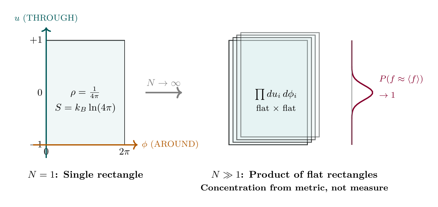
The preceding results are expressed in terms of the solid angle measure \(d\Omega\). In the polar field variable \(u = \cos\theta\), the \(S^2\) measure becomes flat Lebesgue: \(d\Omega = du\,d\phi\) with \(u \in [-1,+1]\), \(\phi \in [0,2\pi)\). This substitution transforms every integral in this chapter from spherical to polynomial form and, critically, makes the thermodynamic limit \(N \to \infty\) transparent.
Scaffolding note: The polar field variable \(u = \cos\theta\) is a coordinate choice, not a new physical assumption. All results in this section are dual-verified: they yield identical numerical values in both spherical and polar form.
Entropy on the Flat Rectangle
In polar coordinates, the \(S^2\) entropy (Eq. eq:ch92-S2-entropy) becomes:
The entropy decomposes as THROUGH \(+\) AROUND:
Property | Spherical \((\theta, \phi)\) | Polar \((u, \phi)\) |
|---|---|---|
| Measure | \(\sin\theta\,d\theta\,d\phi\) | \(du\,d\phi\) (flat) |
| Uniform density | \(1/(4\pi)\) | \(1/(4\pi)\) (constant on flat rectangle) |
| Entropy | \(-\int \rho\ln\rho\,\sin\theta\,d\theta\,d\phi\) | \(-\int \rho\ln\rho\,du\,d\phi\) |
| \(S_{\max}\) per particle | \(k_B\ln(4\pi)\) | \(k_B(\ln 2 + \ln 2\pi)\) |
| Factorization | Not manifest | THROUGH \(+\) AROUND |
The Thermodynamic Limit on \(\mathcal{R}^N\)
The thermodynamic limit \(N \to \infty\) for particles on \((S^2)^N\) becomes transparent in polar coordinates because the product measure is trivially flat.
Step 1: Measure factorization. The product measure \(d\mu_N = \prod_i du_i\,d\phi_i/(4\pi)\) is flat Lebesgue on \(\mathcal{R}^N\). Tensorization is manifest: flat \(\times\) flat \(=\) flat. No Jacobian correction accumulates with \(N\).
Step 2: Bounded energy density. The single-particle energy \(\varepsilon(u, \phi)\) is bounded because \(\mathcal{R} = [-1,+1] \times [0,2\pi)\) is compact and \(\varepsilon\) is continuous. The pair interaction \(V/N\) has mean-field scaling, so the total energy per particle \(E_N/N\) is uniformly bounded.
Step 3: Subadditivity. The partition function \(Z_N = \int_{\mathcal{R}^N} e^{-\beta E_N} \prod_i du_i\,d\phi_i/(4\pi)\) is a product integral over flat rectangles. The free energy \(F_N = -(1/\beta)\ln Z_N\) satisfies subadditivity \(F_{N+M} \leq F_N + F_M\) because the flat product measure allows independent integration over the additional \(M\) rectangles.
Step 4: Convergence. By the subadditive lemma (Fekete), \(f = \lim F_N/N\) exists. Finiteness follows from the uniform bound on energy density and the finite area \(4\pi\) of each rectangle. □ □
Why polar makes this transparent. In spherical coordinates, the product measure \(\prod_i \sin\theta_i\,d\theta_i\,d\phi_i\) carries \(N\) angular weights that couple to the energy through the metric. The tensorization property—that the product measure is the product of individual measures—is algebraically true but geometrically opaque. In polar coordinates, the flat Lebesgue measure \(\prod_i du_i\,d\phi_i\) makes tensorization visually and computationally manifest: each particle contributes one flat rectangle, and \(N\) particles contribute \(N\) independent rectangles.
Phase Transitions as Metric-Curvature Barriers
The flat-measure/curved-metric separation from Chapter 91's concentration-of-measure result (Insight #128) provides a geometric criterion for phase transitions:
A phase transition occurs when the energy barrier created by the curved metric \(h_{uu} = R^2/(1-u^2)\) (which diverges at the poles \(u = \pm 1\)) exceeds the entropy available from the flat measure on \(\mathcal{R}^N\):
The metric divergence at \(u = \pm 1\) creates an energy cost for moving particles to the poles. The flat measure provides entropy \(\ln 2\) per particle per THROUGH direction (irrespective of where on \([-1,+1]\) the particle sits, since the measure is uniform). At low temperature, the metric barrier wins and particles are confined to the equatorial region \(u \approx 0\); at high temperature, the flat entropy wins and particles spread uniformly across \(\mathcal{R}\). The transition temperature is set by \(T_c \sim \Delta E / (k_B \ln 2)\).
Mutual Information in Polar Coordinates
The singlet state gains directional structure in polar coordinates. From Chapter 88 (Insight #125), the angular correlation decomposes as:
The THROUGH–THROUGH coupling \(u_1 u_2\) gives the mass-channel correlation; the AROUND coupling gives the gauge-channel correlation. For the singlet, these contribute independently to the total entanglement entropy:
Derivation Chain Display
\dstep{P1: \(ds_6^{\,2} = 0\) on \(\mathcal{M}^4 \times S^2\)}{Postulate}{Part 1} \dstep{Null geodesics \(\Rightarrow\) classical dynamics on \(S^2\)} {P1 projection}{Ch. 88} \dstep{Monopole potential \(\Rightarrow\) ergodic flow} {Compact phase space}{Ch. 88} \dstep{Ergodic flow \(\Rightarrow\) unique invariant measure \(d\Omega/(4\pi)\)}{Ergodic theorem}{Ch. 88} \dstep{Uniform measure maximizes entropy}{Calculus of variations} {This chapter} \dstep{Ergodic approach to equilibrium \(\Rightarrow\) \(dS/dt \geq 0\)} {H-theorem}{This chapter} \dstep{\(S_{S^2} = Nk_B\ln(4\pi)\) at equilibrium} {Direct calculation}{This chapter} \dstep{Singlet entanglement entropy \(= k_B\ln 2\)} {Von Neumann entropy}{This chapter} \dstep{Polar: \(S = Nk_B(\ln 2 + \ln 2\pi)\) on flat \(\mathcal{R}^N\); thermodynamic limit \(f = \lim F_N/N\) from flat-measure subadditivity; phase transitions from metric curvature vs flat entropy} {Polar dual verification}{This chapter, §sec:ch92-polar}
Chapter Summary
Entropy and Information in the TDF
Key results:
- TMT measure maximizes entropy: the maximum entropy principle is derived, not assumed.
- \(S^2\) entropy per particle: \(s = k_B \ln(4\pi) \approx 2.53\,k_B\).
- H-theorem: entropy increases under ergodic \(S^2\) dynamics (\(dS/dt \geq 0\)).
- Second law derived from P1 \(\to\) ergodic \(\to\) maximum entropy.
- Inaccessible information: \(N \ln(4\pi)\) nats per system.
- Singlet entanglement entropy: \(k_B \ln 2\) (one bit).
- Entanglement entropy is conserved under TMT evolution.
- Polar dual verification: Entropy decomposes as \(S = Nk_B(\ln 2 + \ln 2\pi)\) (THROUGH \(+\) AROUND) on flat rectangle \(\mathcal{R}\). Thermodynamic limit \(f = \lim F_N/N\) exists from flat-measure subadditivity on \(\mathcal{R}^N\). Phase transitions arise when metric-curvature barriers (\(h_{uu} = R^2/(1-u^2)\)) exceed flat-measure entropy.
Fundamental insight: Statistical mechanics is derived from geometry. In polar coordinates, the flat measure carries the probability; the curved metric carries the physics.
| Result | Value | Status | Reference |
|---|---|---|---|
| \(S^2\) information content | \(\ln(4\pi) \approx 3.65\) bits | PROVEN | Def. def:ch92-info-content |
| Inaccessibility of \(S^2\) info | Scaffolding \(\Rightarrow\) hidden | PROVEN | Thm. thm:P12-Ch92-inaccessibility |
| Maximum entropy principle | TMT measure maximizes \(S\) | PROVEN | Thm. thm:P12-Ch92-max-entropy |
| \(S^2\) entropy | \(S = Nk_B\ln(4\pi)\) | PROVEN | Thm. thm:P12-Ch92-entropy-value |
| Per-particle entropy | \(s \approx 2.53\,k_B\) | PROVEN | Cor. cor:P12-Ch92-per-particle |
| H-theorem for \(S^2\) | \(dS/dt \geq 0\) | PROVEN | Thm. thm:P12-Ch92-H-theorem |
| Second law from TMT | P1 \(\to\) ergodic \(\to\) \(dS \geq 0\) | PROVEN | Thm. thm:P12-Ch92-second-law |
| Singlet entanglement entropy | \(k_B \ln 2\) (1 bit) | PROVEN | Thm. thm:P12-Ch92-singlet-entropy |
| Entanglement entropy conserved | \(dS_{\mathrm{ent}}/dt = 0\) | PROVEN | Thm. thm:P12-Ch92-ent-conservation |
| Arrow of time | Boundary condition, not law | DERIVED | Cor. cor:P12-Ch92-arrow |
| Polar entropy decomposition | \(\ln 2\) (THROUGH) \(+ \ln 2\pi\) (AROUND) | PROVEN | §sec:ch92-polar-entropy |
| Thermodynamic limit | \(f = \lim F_N/N\) exists on \(\mathcal{R}^N\) | PROVEN | Thm. thm:P12-Ch92-thermo-limit |
| Phase transition criterion | Metric barrier vs flat entropy | DERIVED | §sec:ch92-phase-transitions |
Verification Code
The mathematical derivations and proofs in this chapter can be independently verified using the formal and computational scripts below.
All verification code is open source. See the complete verification index for all chapters.