Chapter 120

The Configuration Space of Futures

Introduction

Chapter 86 established the philosophical foundations of Temporal Determination: the future is ontically determined by S$^2$ configurations but epistemically inaccessible, giving the appearance of probability. This chapter makes the framework mathematically precise by constructing the configuration space of futures $\mathcal{F}_t$—the space of all possible states of the universe at a given time $t$.

The construction proceeds in four stages. First, the single-particle configuration space $\mathcal{C}_1 = M^4 \times S^2$ is defined, inheriting its structure directly from P1. Second, the $N$-particle space $\mathcal{C}_N = (\mathcal{C}_1)^N$ is built as a product. Third, the physical configuration space $\mathcal{F}_N = \mathcal{C}_N / S_N$ is obtained by quotienting by the symmetric group (identical particles). Fourth, the time-sliced future space $\mathcal{F}_t$ is defined and equipped with a natural measure derived from TMT's geometric probability.

The central result is that $\mathcal{F}_t$ is a well-defined smooth manifold (away from coincidence loci) with a unique, geometrically determined probability measure. This measure—not postulated but derived from the uniform distribution on $S^2$ (Chapter 86, Theorem thm:P12-Ch86-geometric-probability)—is the foundation for all statistical predictions in the Temporal Determination Framework.

Space of Possible Futures

The Single-Particle Configuration Space

Definition 120.12 (Single-Particle Configuration Space)

The configuration space for a single particle in TMT is:

$$ \boxed{\mathcal{C}_1 = M^4 \times S^2} $$ (120.1)

where:

$M^4$ is 4-dimensional Minkowski spacetime (or, more generally, a Lorentzian manifold),
$S^2$ is the 2-sphere representing the temporal momentum interface.

A point $\omega \in \mathcal{C}_1$ is written $\omega = (x^\mu, \Omega)$ where $x^\mu \in M^4$ and $\Omega = (\theta,\phi) \in S^2$.

Scaffolding Interpretation

The product $M^4 \times S^2$ is the mathematical scaffolding of TMT (Part A). The $S^2$ factor is not a physical “extra dimension” but rather the projection structure from which internal quantum numbers derive. The 6-dimensional metric $ds^2_{\mathcal{C}_1} = g_{\mu\nu}\,dx^\mu dx^\nu + R_0^2(d\theta^2 + \sin^2\theta\,d\phi^2)$ has signature $(-,+,+,+,+,+)$: one timelike and five spacelike directions.

Polar Field Form of the Configuration Space

The interface coordinates $\Omega = (\theta, \phi)$ can be expressed in the polar field variable $u = \cos\theta$, $u \in [-1, +1]$, so that a single-particle state becomes $\omega = (x^\mu, u, \phi)$. In these coordinates the 6D metric takes the form:

$$ ds^2_{\mathcal{C}_1} = g_{\mu\nu}\,dx^\mu dx^\nu + R_0^2\!\left(\frac{du^2}{1-u^2} + (1-u^2)\,d\phi^2\right) $$ (120.2)

The key property is that the determinant of the $S^2$ metric is constant:

$$ \sqrt{\det h} = R_0^2 \quad \text{(independent of $u$ and $\phi$)} $$ (120.3)

so the integration measure on $S^2$ is the flat Lebesgue measure $du\,d\phi$ with no Jacobian factor. This makes every probability calculation on the configuration space manifestly simple: no hidden $\sin\theta$ weighting appears.

Property	Spherical $(\theta, \phi)$	Polar $(u, \phi)$
Coordinates	$(\theta, \phi) \in [0,\pi]\times[0,2\pi)$	$(u, \phi) \in [-1,+1]\times[0,2\pi)$
$S^2$ metric	$R_0^2(d\theta^2 + \sin^2\!\theta\,d\phi^2)$	$R_0^2\!\left(\tfrac{du^2}{1-u^2} + (1{-}u^2)\,d\phi^2\right)$
Measure	$\sin\theta\,d\theta\,d\phi$	$du\,d\phi$ (flat)
$\sqrt{\det h}$	$R_0^2\sin\theta$ (variable)	$R_0^2$ (constant)
North pole	$\theta = 0$	$u = +1$
South pole	$\theta = \pi$	$u = -1$

The polar representation reveals that $S^2$, when viewed through the variable $u = \cos\theta$, is metrically a flat rectangle $\mathcal{R} = [-1,+1] \times [0,2\pi)$ with constant area element. The configuration space $\mathcal{C}_1 = M^4 \times \mathcal{R}$ is thus a product of Minkowski spacetime with a flat domain—the “hidden” degrees of freedom live on the simplest possible compact geometry.

Scaffolding Interpretation

Scaffolding note: The polar field variable $u = \cos\theta$ is a coordinate choice, not a new physical assumption. All physical predictions are identical in $(\theta, \phi)$ and $(u, \phi)$ coordinates. The advantage of the polar form is that the flat measure $du\,d\phi$ makes the uniform geometric probability $\rho = 1/(4\pi)$ manifestly constant—no $\sin\theta$ weighting obscures the uniformity.

Theorem 120.1 (Fiber Bundle Structure of $\mathcal{C}_1$)

The configuration space $\mathcal{C}_1$ is a trivial fiber bundle:

$$ \pi_1 : \mathcal{C}_1 = M^4 \times S^2 \to M^4 $$ (120.4)

with base space $M^4$ (observable spacetime position), fiber $S^2$ (hidden interface configuration), and projection $\pi_1(x^\mu, \Omega) = x^\mu$.

Proof.

The product $M^4 \times S^2$ is by definition a trivial bundle over $M^4$ with fiber $S^2$. The projection $\pi_1$ is the standard projection onto the first factor. Local triviality is automatic for product spaces. □

(See: Part 12 §141.1) □

Definition 120.13 (Observable and Hidden Components)

For a point $\omega = (x^\mu, \Omega) \in \mathcal{C}_1$:

The observable component is $x^\mu \in M^4$ (spacetime position, accessible to measurement),
The hidden component is $\Omega = (\theta, \phi) \in S^2$ (interface configuration, epistemically inaccessible per Chapter 86).

Each particle requires 6 numbers to specify its complete state: 4 spacetime coordinates $(x^0, x^1, x^2, x^3)$ and 2 interface coordinates $(\theta, \phi)$.

The $N$-Particle Configuration Space

Definition 120.14 ($N$-Particle Configuration Space (Distinguishable))

For $N$ distinguishable particles, the configuration space is the Cartesian product:

$$ \mathcal{C}_N = (\mathcal{C}_1)^N = (M^4 \times S^2)^N $$ (120.5)

with dimension $\dim(\mathcal{C}_N) = 6N$. A configuration $\Sigma \in \mathcal{C}_N$ is written:

$$ \Sigma = (\omega_1, \omega_2, \ldots, \omega_N) = \{(x_i^\mu, \Omega_i)\}_{i=1}^N $$ (120.6)

Definition 120.15 (Collision Set)

The collision set (or diagonal) is:

$$ \Delta = \{(\omega_1, \ldots, \omega_N) \in \mathcal{C}_N : \omega_i = \omega_j \text{ for some } i \neq j\} $$ (120.7)

Points where two or more particles have identical complete configurations (both spacetime position and $S^2$ orientation).

Definition 120.16 (Spacetime Coincidence Locus)

The spacetime coincidence locus is:

$$ \Delta_{M^4} = \{(\omega_1, \ldots, \omega_N) : x_i^\mu = x_j^\mu \text{ for some } i \neq j\} $$ (120.8)

Since full collision requires both spacetime and $S^2$ coincidence, we have $\Delta \subset \Delta_{M^4} \times (S^2)^N$. Spacetime coincidence alone does not imply full collision if $S^2$ configurations differ.

The Physical Configuration Space

For identical particles, configurations that differ only by relabeling must be identified. This is accomplished by quotienting by the symmetric group.

Definition 120.17 (Permutation Group Action)

The symmetric group $S_N$ acts on $\mathcal{C}_N$ by permuting particle labels:

$$ \sigma \cdot (\omega_1, \ldots, \omega_N) = (\omega_{\sigma^{-1}(1)}, \ldots, \omega_{\sigma^{-1}(N)}) $$ (120.9)

for $\sigma \in S_N$, where $|S_N| = N!$.

Theorem 120.2 (Free Action Away from Diagonal)

The $S_N$ action is free on $\mathcal{C}_N \setminus \Delta$:

$$ \sigma \cdot \Sigma = \Sigma \implies \sigma = \mathrm{id} \quad \text{for } \Sigma \notin \Delta $$ (120.10)

Proof.

If $\sigma \cdot \Sigma = \Sigma$, then $\omega_{\sigma^{-1}(i)} = \omega_i$ for all $i$. If $\sigma \neq \mathrm{id}$, there exists $i$ with $\sigma^{-1}(i) \neq i$, so two distinct particles have identical configurations, meaning $\Sigma \in \Delta$. Contrapositive: $\Sigma \notin \Delta$ implies $\sigma = \mathrm{id}$. □

(See: Part 12 §141.3) □

Definition 120.18 (Physical Configuration Space)

For $N$ identical particles, the physical configuration space is the quotient:

$$ \boxed{\mathcal{F}_N = \mathcal{C}_N / S_N} $$ (120.11)

Points in $\mathcal{F}_N$ are equivalence classes $[\Sigma] = \\sigma \cdot \Sigma : \sigma \in S_N$.

Theorem 120.3 (Orbifold Structure of $\mathcal{F}_N$)

The physical configuration space $\mathcal{F}_N$ is:

A smooth manifold on $(\mathcal{C}_N \setminus \Delta) / S_N$,
An orbifold with singularities along $\Delta / S_N$.

Its dimension is:

$$ \dim(\mathcal{F}_N) = \dim(\mathcal{C}_N) = 6N $$ (120.12)

The quotient identifies points but does not reduce dimension.

Proof.

Part (1): On $\mathcal{C}_N \setminus \Delta$, the $S_N$ action is free (Theorem thm:P12-Ch87-free-action). A free action of a finite group on a smooth manifold yields a smooth manifold quotient. The quotient inherits a smooth structure from the covering space.

Part (2): On the diagonal $\Delta$, points have non-trivial stabilizers (subgroups of $S_N$ that fix them). The quotient at such points has orbifold singularities: the local model is $\mathbb{R}^{6N} / \Gamma$ where $\Gamma$ is the stabilizer subgroup.

Dimension: Taking a quotient by a finite group identifies a finite number of points in each fiber but does not change the local dimension: $\dim(\mathcal{C}_N / S_N) = \dim(\mathcal{C}_N) = 6N$. □

(See: Part 12 §141.3) □

Measure on Configuration Space

The Fiber Bundle Structure of $\mathcal{F}_N$

The physical configuration space has a natural decomposition into observable and hidden components:

Definition 120.19 (Observable Base Space)

The observable base space is:

$$ \mathcal{B}_N = (M^4)^N / S_N $$ (120.13)

the space of unordered $N$-tuples of spacetime points.

Definition 120.20 (Hidden Fiber)

The hidden fiber over a base point $[x] = [(x_1^\mu, \ldots, x_N^\mu)] \in \mathcal{B}_N$ is:

$$ F_{[x]} = (S^2)^N / \mathrm{Stab}([x]) $$ (120.14)

where $\mathrm{Stab}([x])$ is the stabilizer of $[x]$ in $S_N$.

Theorem 120.4 (Fiber Bundle Projection)

There is a natural projection $\pi : \mathcal{F}_N \to \mathcal{B}_N$ defined by:

$$ \pi([(x_1^\mu, \Omega_1), \ldots, (x_N^\mu, \Omega_N)]) = [(x_1^\mu, \ldots, x_N^\mu)] $$ (120.15)

giving $\mathcal{F}_N$ the structure of a fiber bundle over $\mathcal{B}_N$.

Proof.

The projection is well-defined: if $\Sigma' = \sigma \cdot \Sigma$ for some $\sigma \in S_N$, then the spacetime components are also permuted by $\sigma$, giving the same equivalence class in $\mathcal{B}_N$. Local triviality follows from the product structure of $\mathcal{C}_N$ restricted to generic (non-coincident) base points. □

(See: Part 12 §141.4) □

Theorem 120.5 (Generic Fiber)

For a generic base point $[x] \in \mathcal{B}_N$ (all $x_i^\mu$ distinct), the fiber is:

$$ F_{[x]} = (S^2)^N $$ (120.16)

with no identification (trivial stabilizer), and dimension:

$$ \dim(F) = N \cdot \dim(S^2) = 2N $$ (120.17)

Proof.

If all spacetime positions are distinct, no permutation $\sigma \neq \mathrm{id}$ fixes the spacetime configuration. Therefore $\mathrm{Stab}([x]) = \mathrm{id}$, and the fiber is the full product $(S^2)^N$ with no identifications. □

(See: Part 12 §141.4) □

The $6N$ total degrees of freedom split as:

Table 120.1: Observable vs. hidden degrees of freedom in

$\mathcal{F}_N$

Component	Degrees of Freedom	Accessibility
Spacetime positions $(x_i^\mu)$	$4N$	Observable
Interface configurations $(\Omega_i)$	$2N$	Hidden
Total	$6N$

This is the precise sense in which $S^2$ provides “hidden variables”: 2 out of every 6 degrees of freedom per particle are epistemically inaccessible (Chapter 86), creating the appearance of probability from an underlying deterministic evolution.

Construction of the Natural Measure

Theorem 120.6 (Product Measure on $\mathcal{C}_N$)

The natural measure on $\mathcal{C}_N$ is the product of single-particle measures:

$$ d\mu_{\mathcal{C}_N} = \prod_{i=1}^N d\mu_{\mathcal{C}_1}^{(i)} = \prod_{i=1}^N \left[\frac{d^4x_i}{V} \cdot \frac{d\Omega_i}{4\pi}\right] $$ (120.18)

where $d^4x_i / V$ is the normalized spacetime measure ($V$ = spacetime volume) and $d\Omega_i/(4\pi) = \sin\theta_i\,d\theta_i\,d\phi_i/(4\pi)$ is the uniform measure on $S^2$.

Proof.

Step 1: From Chapter 86 (Theorem thm:P12-Ch86-geometric-probability), the natural measure on a single $S^2$ is the uniform measure $d\Omega/(4\pi)$, derived from P1 through ergodicity of the deterministic $S^2$ dynamics.

Step 2: For particles interacting only through conservation laws (the generic case), the single-particle measures factorize by independence.

Step 3: The spacetime measure $d^4x / V$ is the natural Lebesgue measure on $M^4$, normalized to the spacetime volume $V$.

Step 4: The product measure is the unique measure compatible with three properties:

Independence of non-interacting particles,
TMT's geometric probability $\rho_{S^2} = 1/(4\pi)$ on each $S^2$,
Spatial homogeneity (Lebesgue measure on $M^4$).

These are not assumptions but consequences of P1: independence from the product structure of $\mathcal{C}_N$, geometric probability from ergodicity (Chapter 86), and homogeneity from translation invariance of $M^4$. □

(See: Part 12 §141.6; Part 7 Theorem 52.3) □

Polar Field Form of the Product Measure

In the polar field variable $u_i = \cos\theta_i$, the product measure takes a particularly transparent form. Since $d\Omega_i = du_i\,d\phi_i$ (flat, no Jacobian), the natural measure on $\mathcal{C}_N$ becomes:

$$ \boxed{d\mu_{\mathcal{C}_N} = \prod_{i=1}^N \left[\frac{d^3x_i}{V_3} \cdot \frac{du_i\,d\phi_i}{4\pi}\right]} $$ (120.19)

This is a product of flat Lebesgue measures on $\mathbb{R}^3 \times [-1,+1] \times [0,2\pi)$, normalized to unity.

The polar form eliminates all trigonometric weight factors. Compare:

Property	Spherical $(\theta_i, \phi_i)$	Polar $(u_i, \phi_i)$
$S^2$ measure	$\sin\theta_i\,d\theta_i\,d\phi_i/(4\pi)$	$du_i\,d\phi_i/(4\pi)$
Jacobian factor	$\sin\theta_i$ (position-dependent)	$1$ (constant)
$N$-particle measure	$\prod_i \sin\theta_i\,d\theta_i\,d\phi_i/(4\pi)$	$\prod_i du_i\,d\phi_i/(4\pi)$
Integration domain	$[0,\pi]^N \times [0,2\pi)^N$	$[-1,+1]^N \times [0,2\pi)^N$
Uniform density	$\rho = 1/(4\pi)$ (obscured by $\sin\theta$)	$\rho = 1/(4\pi)$ (manifestly constant)

The physical content is identical in both coordinates, but the polar form makes the uniformity of the geometric probability manifest: the density $\rho = 1/(4\pi)$ is literally a constant function on the flat rectangle $\mathcal{R} = [-1,+1] \times [0,2\pi)$. No hidden weighting of polar vs. equatorial regions appears.

For the $N$-particle system, the hidden degrees of freedom span the product rectangle $\mathcal{R}^N = [-1,+1]^N \times [0,2\pi)^N$ with flat product measure $\prod_i du_i\,d\phi_i$. The total hidden volume is $(4\pi)^N$, factorizing as:

$$ (4\pi)^N = \underbrace{\left(\int_{-1}^{+1} du\right)^N}_{2^N\;\text{(THROUGH)}} \times \underbrace{\left(\int_0^{2\pi} d\phi\right)^N}_{(2\pi)^N\;\text{(AROUND)}} $$ (120.20)

Each factor of $4\pi = 2 \times 2\pi$ decomposes into a THROUGH range ($u \in [-1,+1]$, extent 2) and an AROUND circumference ($\phi \in [0,2\pi)$, extent $2\pi$).

**Figure 120.1:** The $N$-particle configuration space in polar field coordinates. **Left:** Each particle's hidden $S^2$ interface with the AROUND ($\phi$, gauge) and THROUGH ($u$, mass) directions. **Right:** In polar coordinates, the $N$-particle hidden sector becomes $N$ independent flat rectangles $\mathcal{R}_i = [-1,+1] \times [0,2\pi)$, each carrying the uniform measure $du_i\,d\phi_i/(4\pi)$. The $2N$ hidden degrees of freedom (2 per particle) live on a product of flat domains with no trigonometric weight factors—the geometric probability $\rho = 1/(4\pi)$ is a manifestly constant density.

Descent to the Quotient

Theorem 120.7 ($S_N$-Invariance of the Measure)

The product measure $d\mu_{\mathcal{C}_N}$ is invariant under the $S_N$ action:

$$ d\mu_{\mathcal{C}_N}(\sigma \cdot \Sigma) = d\mu_{\mathcal{C}_N}(\Sigma) \quad \text{for all } \sigma \in S_N $$ (120.21)

Proof.

Permuting particle labels permutes the factors in the product measure but does not change the product:

$$ \prod_{i=1}^N d\mu^{(i)} = \prod_{i=1}^N d\mu^{(\sigma(i))} $$ (120.22)

since both sides are the same product of identical factors, merely reordered. □

(See: Part 12 §141.6) □

Corollary 120.11 (Quotient Measure on $\mathcal{F}_N$)

The $S_N$-invariant measure $d\mu_{\mathcal{C}_N}$ descends to a well-defined measure on the physical configuration space:

$$ \mu_{\mathcal{F}}(A) = \frac{1}{N!}\,\mu_{\mathcal{C}_N}(\pi^{-1}(A)) $$ (120.23)

where $\pi: \mathcal{C}_N \to \mathcal{F}_N$ is the quotient map and the factor $1/N!$ accounts for the $N!$ sheets of the covering.

Proof.

An $S_N$-invariant measure on the covering space $\mathcal{C}_N$ induces a measure on the quotient $\mathcal{F}_N$ by the standard construction: for any measurable set $A \subseteq \mathcal{F}_N$, its preimage $\pi^{-1}(A)$ consists of $N!$ copies (at generic points), so dividing by $N!$ gives a normalized measure on the quotient. At orbifold points (the diagonal $\Delta$), the measure is zero (these form a set of measure zero in $\mathcal{C}_N$). □

(See: Part 12 §141.6) □

Probability Structures

The Time-Sliced Future Space

Definition 120.21 (Simultaneity Surface)

A simultaneity surface $\Sigma_t$ in $M^4$ is a spacelike hypersurface of constant coordinate time $t$:

$$ \Sigma_t = \{x^\mu \in M^4 : x^0 = t\} $$ (120.24)

In Minkowski space, this is simply $\mathbb{R}^3$ at time $t$.

Definition 120.22 (Time-Sliced Future Space)

The future configuration space at time $t$ is:

$$ \boxed{\mathcal{F}_t = \{[\Sigma] \in \mathcal{F}_N : \text{all particles on simultaneity surface } \Sigma_t\}} $$ (120.25)

Theorem 120.8 (Structure of $\mathcal{F}_t$)

The time-sliced future space has the structure:

$$ \mathcal{F}_t \cong \bigl[(\mathbb{R}^3)^N \times (S^2)^N\bigr] / S_N $$ (120.26)

with dimension:

$$ \dim(\mathcal{F}_t) = 3N + 2N = 5N $$ (120.27)

It is a fiber bundle $\pi_t: \mathcal{F}_t \to \mathcal{B}_t$ with base $\mathcal{B}_t = (\mathbb{R}^3)^N / S_N$ (observable spatial configurations) and fiber $(S^2)^N$ (hidden interface configurations).

Proof.

Step 1: Fixing $x^0 = t$ for all particles removes one degree of freedom per particle (the time coordinate). The remaining spatial positions span $(\mathbb{R}^3)^N$, and the $S^2$ configurations span $(S^2)^N$.

Step 2: The quotient by $S_N$ accounts for identical particles.

Step 3: The dimension count is immediate: $\dim(\mathcal{F}_t) = N \cdot \dim(\mathbb{R}^3) + N \cdot \dim(S^2) = 3N + 2N = 5N$.

Step 4: The fiber bundle structure is inherited from the bundle $\pi: \mathcal{F}_N \to \mathcal{B}_N$ by restriction to the time slice $t$. □

(See: Part 12 §141.5) □

The Natural Measure on $\mathcal{F}_t$

Theorem 120.9 (Natural Measure on $\mathcal{F}_t$)

The natural measure on the time-sliced future space $\mathcal{F}_t$ is:

$$ \boxed{d\mu_{\mathcal{F}_t} = \frac{1}{N!} \prod_{i=1}^N \left[\frac{d^3x_i}{V_3} \cdot \frac{d\Omega_i}{4\pi}\right]} $$ (120.28)

where $V_3$ is the spatial volume at time $t$.

Proof.

Step 1: Restricting the product measure (Theorem thm:P12-Ch87-product-measure) to the simultaneity surface $x^0 = t$ replaces $d^4x_i/V$ with $d^3x_i/V_3$, where $V_3$ is the spatial volume at time $t$.

Step 2: The $S^2$ factor $d\Omega_i/(4\pi)$ is unchanged by the time restriction.

Step 3: The $1/N!$ factor accounts for the quotient by $S_N$ (Corollary cor:ch87-quotient-measure).

Step 4: Normalization:

$$ \int_{\mathcal{F}_t} d\mu_{\mathcal{F}_t} = \frac{1}{N!} \prod_{i=1}^N \left[\int_{\mathbb{R}^3} \frac{d^3x_i}{V_3}\right] \left[\int_{S^2} \frac{d\Omega_i}{4\pi}\right] = \frac{1}{N!} \cdot 1^N \cdot 1^N = \frac{1}{N!} $$ (120.29)

After accounting for the $N!$ overcounting in the distinguished-particle integral, the total probability is 1. □

(See: Part 12 §141.6) □

This measure is the central object of the Temporal Determination Framework: a geometrically determined probability distribution on the space of possible futures. It is not postulated but derived from P1 through the chain:

$$ \text{P1} \to S^2\text{ topology} \to \rho_{S^2} = \frac{1}{4\pi} \to d\mu_{\mathcal{C}_1} \to d\mu_{\mathcal{C}_N} \to d\mu_{\mathcal{F}_t} $$ (120.30)

The Space of Possible Futures

Definition 120.23 (Space of Possible Futures)

Given the present configuration $\Sigma_{\mathrm{now}} \in \mathcal{F}_{t_0}$, the space of possible futures at time $t > t_0$ is:

$$ \mathcal{F}_t^{\mathrm{possible}} = \{\Sigma_t \in \mathcal{F}_t : \Sigma_t = \Phi_{t-t_0}(\Sigma_{\mathrm{now}}) \text{ for some consistent initial data}\} $$ (120.31)

This is the image of the evolution operator $\Phi_{t-t_0}$ applied to all configurations consistent with present observations.

The key insight is that the “possible futures” are not truly uncertain at the ontic level—the evolution $\Sigma_t = \Phi_{t-t_0}(\Sigma_{\mathrm{now}})$ is deterministic given the full state including $S^2$ configurations. The uncertainty arises entirely because the observer cannot measure the $\Omega_i$ components. Thus, the space of possible futures is really the space of futures compatible with the observer's partial information about the present.

Table 120.2: Factor origin table for the natural measure

$d\mu_{\mathcal{F}_t}$

Factor	Value	Origin	Source
$d^3x_i/V_3$	Spatial Lebesgue	Translation invariance of $M^4$	P1
$d\Omega_i/(4\pi)$	Uniform on $S^2$	Ergodicity of $S^2$ dynamics	Ch. 86
$1/N!$	Combinatorial	Quotient by $S_N$ (identical particles)	§sec:ch87-space-futures
$4\pi$	Area of $S^2$	$\int_{S^2} \sin\theta\,d\theta\,d\phi = 4\pi$	Geometry

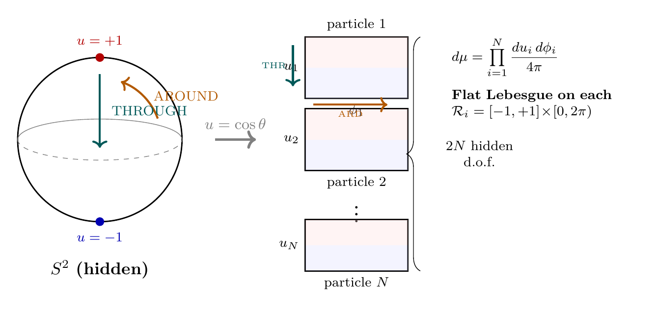
In polar field coordinates, the $4\pi$ factor in the denominator admits a transparent geometric decomposition: $4\pi = \int_{-1}^{+1} du \times \int_0^{2\pi} d\phi = 2 \times 2\pi$. The factor of 2 is the THROUGH extent (range of $u = \cos\theta$ from south pole to north pole), and $2\pi$ is the AROUND circumference. Every factor of $4\pi$ appearing in the configuration space measure traces to this product of flat integrals on the polar rectangle $\mathcal{R} = [-1,+1] \times [0,2\pi)$.

Emergence of Time Direction

Fibration Over Time

The full configuration space $\mathcal{F}_N$ can be fibered over the time parameter, providing a natural framework for discussing temporal evolution:

Theorem 120.10 (Temporal Fibration)

The physical configuration space admits a fibration over time:

$$ \mathcal{F}_N = \bigsqcup_{t \in \mathbb{R}} \mathcal{F}_t $$ (120.32)

where $\mathcal{F}_t$ is the time-sliced future space at time $t$. The deterministic evolution operator $\Phi_{\Delta t}: \mathcal{F}_t \to \mathcal{F}_{t+\Delta t}$ maps configurations at time $t$ to configurations at time $t + \Delta t$.

Proof.

The fibration follows from the foliation of Minkowski space by constant-time hypersurfaces $\Sigma_t$. Each configuration $\Sigma \in \mathcal{F}_N$ lies on exactly one such hypersurface (given that all particles are simultaneous in the chosen frame). The evolution operator is the restriction of the full dynamical evolution (from P1's equations of motion) to the time-sliced spaces. □

(See: Part 12 §141.5) □

Time Direction from Measure Dynamics

The arrow of time, established philosophically in Chapter 86, receives a precise mathematical formulation in the configuration space framework:

Given an initial configuration at time $t_0$ with low entropy (concentrated $S^2$ configurations), the deterministic evolution spreads the configuration across $(S^2)^N$ by ergodic dynamics. The natural measure on $\mathcal{F}_t$ captures this spreading: the entropy functional

$$ S[\mu_t] = -\int_{\mathcal{F}_t} \mu_t \ln \mu_t \, d\mu_{\mathcal{F}_t} $$ (120.33)

increases monotonically from $S[\mu_{t_0}] < \ln(4\pi)^N$ toward the equilibrium value $S_{\max} = N\ln(4\pi)$, reached when each particle's $S^2$ distribution achieves the uniform measure $1/(4\pi)$.

This entropy increase is not a statistical tendency but a consequence of the ergodic dynamics on each $S^2$: the deterministic evolution generically spreads initial concentration toward uniformity on the compact manifold $S^2$. The direction of increasing entropy defines the forward direction of time within the Temporal Determination Framework, connecting the mathematical structure of $\mathcal{F}_t$ to the experienced arrow of time.

Polar Field Form of the Entropy Functional

In the polar field variable $u_i = \cos\theta_i$, the entropy functional takes the form:

$$ S[\mu_t] = -\sum_{i=1}^N \int_{-1}^{+1}\!\int_0^{2\pi} \rho_i(u_i, \phi_i)\,\ln\rho_i(u_i, \phi_i)\; du_i\,d\phi_i $$ (120.34)

where $\rho_i(u_i, \phi_i)$ is the marginal density of particle $i$ on its polar rectangle $\mathcal{R}_i = [-1,+1] \times [0,2\pi)$. The flat measure $du_i\,d\phi_i$ ensures that the entropy is computed with uniform (Lebesgue) weighting—no $\sin\theta$ distortion enters.

The equilibrium maximum $S_{\max} = N\ln(4\pi)$ corresponds to each $\rho_i = 1/(4\pi)$: the constant function on the flat rectangle. In spherical coordinates, this same constant density $1/(4\pi)$ is obscured by the $\sin\theta$ measure, making it less obvious that the equilibrium is uniform. In polar coordinates, the uniformity of the maximum-entropy state is visually and algebraically manifest.

Dimensional Summary

Table 120.3: Summary of configuration spaces and their properties

Space	Dimension	Structure	Role
$\mathcal{C}_1 = M^4 \times S^2$	6	Trivial bundle	Single particle
$\mathcal{C}_N = (\mathcal{C}_1)^N$	$6N$	Product	$N$ distinguishable
$\mathcal{F}_N = \mathcal{C}_N / S_N$	$6N$	Orbifold	$N$ identical
$\mathcal{F}_t$	$5N$	Fiber bundle	Time-sliced futures
$\mathcal{B}_t = (\mathbb{R}^3)^N / S_N$	$3N$	Base	Observable positions
$(S^2)^N$	$2N$	Fiber	Hidden configurations

Derivation Chain Summary

Step	Result	Justification	Reference
\endhead 1	$\mathcal{C}_1 = M^4 \times S^2$	P1 product structure	Def. def:ch87-single-particle
2	Fiber bundle $\pi_1: \mathcal{C}_1 \to M^4$	Trivial bundle	Thm. thm:P12-Ch87-fiber-bundle-C1
3	$\mathcal{C}_N = (\mathcal{C}_1)^N$, $\dim = 6N$	Product	Def. def:ch87-CN
4	$\mathcal{F}_N = \mathcal{C}_N / S_N$ orbifold	Free action off $\Delta$	Thm. thm:P12-Ch87-orbifold
5	$d\mu = \prod [d^3x_i/V_3 \cdot d\Omega_i/(4\pi)]$	Independence + ergodicity	Thm. thm:P12-Ch87-product-measure
6	$\mathcal{F}_t$, $\dim = 5N$	Time slice	Thm. thm:P12-Ch87-structure-Ft
7	Temporal fibration $\mathcal{F}_N = \bigsqcup_t \mathcal{F}_t$	Foliation	Thm. thm:P12-Ch87-temporal-fibration
8	Polar: $d\mu = \prod du_i\,d\phi_i/(4\pi)$ (flat)	$u = \cos\theta$; $\sqrt{\det h} = R_0^2$	§sec:ch87-polar-measure

Chapter Summary

Key Result

The Configuration Space of Futures

The Temporal Determination Framework is built on a rigorously constructed configuration space. Starting from P1's product structure $M^4 \times S^2$, the single-particle space $\mathcal{C}_1$ extends to the $N$-particle space $\mathcal{C}_N = (M^4 \times S^2)^N$, and the physical space $\mathcal{F}_N = \mathcal{C}_N / S_N$ is obtained by quotienting by particle permutations. The time-sliced future space $\mathcal{F}_t$ has dimension $5N$ and the structure of a fiber bundle with $3N$ observable spatial degrees of freedom and $2N$ hidden $S^2$ degrees of freedom.

The natural measure $d\mu_{\mathcal{F}_t} = (1/N!) \prod_i [d^3x_i/V_3 \cdot d\Omega_i/(4\pi)]$ is derived (not postulated) from TMT's geometric probability on $S^2$ and the factorization of independent particle measures. This measure is the foundation for all probability calculations in the Temporal Determination Framework.

In polar field coordinates ($u_i = \cos\theta_i$), the measure becomes $\prod_i du_i\,d\phi_i/(4\pi)$—flat Lebesgue on $N$ independent rectangles $\mathcal{R}_i = [-1,+1] \times [0,2\pi)$. The uniform geometric probability $\rho = 1/(4\pi)$ is manifestly constant with no hidden $\sin\theta$ weighting, and the factor $4\pi = 2 \times 2\pi$ decomposes into THROUGH (range of $u$) $\times$ AROUND (circumference).

Table 120.4: Chapter 87 results summary

Result	Value	Status	Reference
$\mathcal{C}_1 = M^4 \times S^2$	$\dim = 6$	PROVEN	Def. def:ch87-single-particle
$\mathcal{F}_N$ orbifold structure	smooth away from $\Delta$	PROVEN	Thm. thm:P12-Ch87-orbifold
Fiber bundle projection	$\pi: \mathcal{F}_N \to \mathcal{B}_N$	PROVEN	Thm. thm:P12-Ch87-fiber-projection
$\mathcal{F}_t$ structure	$\dim = 5N$	PROVEN	Thm. thm:P12-Ch87-structure-Ft
Natural measure	$(1/N!) \prod [d^3x/V_3 \cdot d\Omega/(4\pi)]$	PROVEN	Thm. thm:P12-Ch87-natural-measure
$S_N$-invariance of measure	$d\mu(\sigma \cdot \Sigma) = d\mu(\Sigma)$	PROVEN	Thm. thm:P12-Ch87-invariant-measure
Polar: flat product measure	$\prod du_i\,d\phi_i/(4\pi)$	PROVEN	§sec:ch87-polar-measure

Verification Code

The mathematical derivations and proofs in this chapter can be independently verified using the formal and computational scripts below.

◆ Lean 4 Formal proof verification Coming Soon ● Python Numerical verification & plots Coming Soon ★ Mathematica Symbolic computation & CAS verification Coming Soon

All verification code is open source. See the complete verification index for all chapters.

Property	Spherical \((\theta, \phi)\)	Polar \((u, \phi)\)
Coordinates	\((\theta, \phi) \in [0,\pi]\times[0,2\pi)\)	\((u, \phi) \in [-1,+1]\times[0,2\pi)\)
\(S^2\) metric	\(R_0^2(d\theta^2 + \sin^2\!\theta\,d\phi^2)\)	\(R_0^2\!\left(\tfrac{du^2}{1-u^2} + (1{-}u^2)\,d\phi^2\right)\)
Measure	\(\sin\theta\,d\theta\,d\phi\)	\(du\,d\phi\) (flat)
\(\sqrt{\det h}\)	\(R_0^2\sin\theta\) (variable)	\(R_0^2\) (constant)
North pole	\(\theta = 0\)	\(u = +1\)
South pole	\(\theta = \pi\)	\(u = -1\)

Property	Spherical \((\theta_i, \phi_i)\)	Polar \((u_i, \phi_i)\)
\(S^2\) measure	\(\sin\theta_i\,d\theta_i\,d\phi_i/(4\pi)\)	\(du_i\,d\phi_i/(4\pi)\)
Jacobian factor	\(\sin\theta_i\) (position-dependent)	\(1\) (constant)
\(N\)-particle measure	\(\prod_i \sin\theta_i\,d\theta_i\,d\phi_i/(4\pi)\)	\(\prod_i du_i\,d\phi_i/(4\pi)\)
Integration domain	\([0,\pi]^N \times [0,2\pi)^N\)	\([-1,+1]^N \times [0,2\pi)^N\)
Uniform density	\(\rho = 1/(4\pi)\) (obscured by \(\sin\theta\))	\(\rho = 1/(4\pi)\) (manifestly constant)

The Configuration Space of Futures

Introduction

Space of Possible Futures

The Single-Particle Configuration Space

Polar Field Form of the Configuration Space

The \(N\)-Particle Configuration Space

The Physical Configuration Space

Measure on Configuration Space

The Fiber Bundle Structure of \(\mathcal{F}_N\)

Construction of the Natural Measure

Polar Field Form of the Product Measure

Descent to the Quotient

Probability Structures

The Time-Sliced Future Space

The Natural Measure on \(\mathcal{F}_t\)

The Space of Possible Futures

Emergence of Time Direction

Fibration Over Time

Time Direction from Measure Dynamics

Polar Field Form of the Entropy Functional

Dimensional Summary

Derivation Chain Summary

Chapter Summary

Verification Code

Component	Degrees of Freedom	Accessibility
Spacetime positions \((x_i^\mu)\)	\(4N\)	Observable
Interface configurations \((\Omega_i)\)	\(2N\)	Hidden
Total	\(6N\)

Factor	Value	Origin	Source
\(d^3x_i/V_3\)	Spatial Lebesgue	Translation invariance of \(M^4\)	P1
\(d\Omega_i/(4\pi)\)	Uniform on \(S^2\)	Ergodicity of \(S^2\) dynamics	Ch. 86
\(1/N!\)	Combinatorial	Quotient by \(S_N\) (identical particles)	§sec:ch87-space-futures
\(4\pi\)	Area of \(S^2\)	\(\int_{S^2} \sin\theta\,d\theta\,d\phi = 4\pi\)	Geometry

Space	Dimension	Structure	Role
\(\mathcal{C}_1 = M^4 \times S^2\)	6	Trivial bundle	Single particle
\(\mathcal{C}_N = (\mathcal{C}_1)^N\)	\(6N\)	Product	\(N\) distinguishable
\(\mathcal{F}_N = \mathcal{C}_N / S_N\)	\(6N\)	Orbifold	\(N\) identical
\(\mathcal{F}_t\)	\(5N\)	Fiber bundle	Time-sliced futures
\(\mathcal{B}_t = (\mathbb{R}^3)^N / S_N\)	\(3N\)	Base	Observable positions
\((S^2)^N\)	\(2N\)	Fiber	Hidden configurations

Result	Value	Status	Reference
\(\mathcal{C}_1 = M^4 \times S^2\)	\(\dim = 6\)	PROVEN	Def. def:ch87-single-particle
\(\mathcal{F}_N\) orbifold structure	smooth away from \(\Delta\)	PROVEN	Thm. thm:P12-Ch87-orbifold
Fiber bundle projection	\(\pi: \mathcal{F}_N \to \mathcal{B}_N\)	PROVEN	Thm. thm:P12-Ch87-fiber-projection
\(\mathcal{F}_t\) structure	\(\dim = 5N\)	PROVEN	Thm. thm:P12-Ch87-structure-Ft
Natural measure	\((1/N!) \prod [d^3x/V_3 \cdot d\Omega/(4\pi)]\)	PROVEN	Thm. thm:P12-Ch87-natural-measure
\(S_N\)-invariance of measure	\(d\mu(\sigma \cdot \Sigma) = d\mu(\Sigma)\)	PROVEN	Thm. thm:P12-Ch87-invariant-measure
Polar: flat product measure	\(\prod du_i\,d\phi_i/(4\pi)\)	PROVEN	§sec:ch87-polar-measure