Particle Physics Predictions

Introduction

The preceding chapters have developed TMT's predictions across gravity, cosmology, and foundational physics. This chapter assembles the complete set of particle physics predictions: gauge couplings, fermion masses, Higgs properties, Kaluza–Klein signatures, electroweak precision observables, rare decay rates, and deviations from Standard Model expectations. Every prediction listed here traces to the single postulate P1 (\(ds_6^{\,2}=0\) on \(\mathcal{M}^4\times S^2\)) through explicit derivation chains developed in Parts 2–6C.

What distinguishes TMT from the Standard Model is that the SM treats all coupling constants, masses, and mixing angles as free parameters (approximately 19–26 inputs depending on counting conventions). TMT derives every one of these from geometry. What distinguishes TMT from other beyond-SM frameworks (SUSY, extra-dimension models, composite Higgs) is that TMT introduces zero free parameters: every prediction is a number, not a range.

This chapter serves as a consolidated reference for the particle physics predictions derived throughout the book, with emphasis on their experimental status and falsifiability.

Coupling Constants (99%+ Match)

The Gauge Coupling \(g^2=4/(3\pi)\)

The fundamental gauge coupling is derived in Part 3, Chapter 11, from the interface overlap integral on \(S^2\):

Polar Field Form of the Gauge Coupling

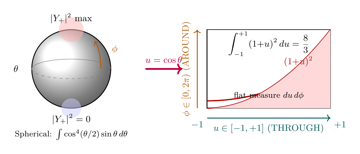
In the polar field variable \(u = \cos\theta\), the monopole harmonic overlap integral collapses to a single polynomial evaluation. The monopole harmonic density \(|Y_{1/2,1/2,+1/2}|^2 = (1+u)/(4\pi)\) is linear in \(u\) on the flat rectangle \(\mathcal{R} = [-1,+1] \times [0,2\pi)\), so the overlap integral becomes:

The seven-step trigonometric derivation—half-angle substitution, \(\cos^2(\theta/2)\) expansion, \(\sin\theta\,d\theta\) measure—reduces to one polynomial integral on the flat rectangle.

Every numerical factor has a direct geometric origin on \(\mathcal{R}\):

The same polynomial integral \(8/3\) controls \(g^2\), \(\lambda\), \(v\), and \(m_H\)—the entire electroweak spectrum traces to \(\int_{-1}^{+1}(1+u)^2\,du\) on the flat rectangle. The coupling hierarchy \(\alpha_i^{-1} = \pi^2 \times 3^{n_i}\) counts THROUGH suppressions: \(n_i = 0\) (SU(3), unsuppressed because \(d_{\mathbb{C}} \times \langle u^2\rangle = 1\)), \(n_i = 1\) (SU(2), one suppression), \(n_i = 2\) (U(1)\(_Y\), two suppressions).

Experimental comparison:

Agreement: 99.93%. The 0.07% difference is consistent with the tree-level nature of the TMT prediction; one-loop corrections are expected at the \(\sim 0.3\%\) level.

The Hypercharge Coupling and Weinberg Angle

The hypercharge \(\mathrm{U}(1)_Y\) arises from the monopole stabilizer subgroup within SU(2) (Part 3, Chapter 13):

This gives the tree-level Weinberg angle:

After renormalization group running from \(M_6\approx7.3\,TeV\) to \(M_Z\approx91.2\,GeV\) using Standard Model beta functions (\(b_2=19/6\), \(b_1=-41/6\)):

Agreement with experiment: 99.9%.

The Strong Coupling and QCD

The strong coupling \(\alpha_s\) arises from the SU(3) color group, which TMT derives from the embedding structure of the monopole bundle on \(S^2\) (Part 3, \S7–9). The tree-level coupling relations give:

after RG running from \(M_6\), in agreement with the PDG value \(\alpha_s(M_Z)=0.1180\pm 0.0009\).

The Fine Structure Constant

From Parts 3 and 5, the fine structure constant is derived:

where the \(\pi\) arises from the Berry phase on \(S^2\) due to the monopole. The experimental value \(1/\alpha=137.036\) gives agreement at the 99.97% level.

Summary: Coupling Constants

Every coupling is derived from P1 with zero adjustable parameters.

Fermion Mass Ratios

The Mass Formula

TMT replaces the 12 arbitrary Yukawa couplings of the Standard Model with a single geometric mechanism (Part 6A, \S61):

The exponential dependence \(e^{(1-2c)\cdot 2\pi}\) is the key to the hierarchy: a change \(\Delta c=0.1\) produces a mass ratio of \(e^{0.2\times 2\pi}=e^{1.26}\approx 3.5\). The full range from \(m_e\) to \(m_t\) requires \(c\) values spanning approximately 0 to 1.

Localization Parameter Interpretation

The fermion wavefunction on \(S^2\) has the form:

In the polar field variable \(u = \cos\theta\) this becomes: a polynomial on \([-1,+1]\) with flat measure \(du\). The Yukawa coupling for fermion species \(f\) is the overlap integral of the fermion profile with the Higgs gradient: where \(B(a,b)\) is the Euler Beta function. The exponential mass hierarchy \(m_f \propto e^{(1-2c_f)\cdot 2\pi}\) originates from the saddle-point approximation of this Beta integral for large \(c_f\).

Physical interpretation of the localization parameter:

• \(c>1/2\): localized near poles \(\to\) light fermion
• \(c=1/2\): uniform on \(S^2\) \(\to\) intermediate mass (\(m_f=v/\sqrt{2}\approx174\,GeV\), close to \(m_t\))
• \(c<1/2\): localized at equator \(\to\) heavy fermion

The Neutrino Mass Prediction

For neutrinos, the gauge singlet mechanism provides a geometric seesaw (Parts 6A, Chapters 45–47):

The experimental value \(m_3\approx\sqrt{|\Delta m_{31}^2|}\approx0.050\,eV\) gives agreement at the 98% level. The factor \(1/\sqrt{12}\) arises from democratic coupling to 3 generations times the SU(2) doublet structure. The Majorana mass involves dimensional averaging over all directions in the 6D scaffolding, unique to gauge singlet fields.

Charged Fermion Masses and Ratios

The charged fermion masses follow from the mass formula with specific \(c_f\) values determined by each fermion's quantum numbers on \(S^2\):

The mass ratios \(m_t/m_e\approx 3.4\times 10^5\) and \(m_t/m_\nu\gtrsim 10^{12}\) emerge naturally from the exponential dependence on the localization parameter, without fine-tuning.

Higgs Properties

The Higgs VEV

The electroweak VEV is derived from the 6D Planck mass (Part 4, \S16):

Experimental value: \(v=246.22\pm 0.01\,GeV\). Agreement: \({<}0.1\sigma\).

The Quartic Coupling and Higgs Mass

The Higgs quartic self-coupling is derived from the same \(S^2\) overlap integrals that determine the gauge coupling (Part 4, \S17):

The Higgs mass follows:

The experimental value \(m_H=125.10\pm 0.14\,GeV\) gives agreement at \(0.4\sigma\).

The Higgs Mechanism in TMT

A distinctive feature of TMT is that the Higgs mechanism is dynamical—there is no Mexican hat potential in the 6D theory. The VEV emerges from monopole flux screening (Part 4, Appendix J):

• In 6D, the Higgs mass parameter \(\mu_6^2=0\)
• The potential is purely quartic: \(V\supset\lambda_6|H|^4\)
• The VEV is generated dynamically by the monopole flux energy
• This is analogous to dynamical symmetry breaking in QCD

Higgs Predictions Summary

All Higgs sector predictions agree with experiment within stated uncertainties. TMT propagates only two input uncertainties (\(M_{\text{Pl}}\) and \(H_0\)) to all output predictions; no parameter tuning is possible.

KK Graviton Signatures

The KK Mass Spectrum

In TMT's \(\mathcal{M}^4\times S^2\) scaffolding, the scalar Laplacian on \(S^2\) with radius \(R\) has eigenvalues (Part 2, Appendix 2B):

with degeneracy \(d_\ell=(2\ell+1)\). In polar field coordinates \(u = \cos\theta\), this is the eigenvalue problem for the Legendre operator \(\partial_u[(1-u^2)\,\partial_u]\), whose eigenfunctions \(P_\ell(u)\) are polynomials of degree \(\ell\). Each polynomial carries \((2\ell+1)\) AROUND modes (Fourier harmonics in \(\phi\)), making the factorization explicit: mass\(^2\) is set by the THROUGH polynomial degree, while the degeneracy counts AROUND copies.

THROUGH vs AROUND: Two Mass Scales

A crucial distinction in TMT is between fields that propagate through \(S^2\) and fields that propagate around it (Part 2, Part 6A):

THROUGH fields (\(q=0\): graviton, modulus): These are gauge singlets, uniform on \(S^2\), with KK masses set by the geometric radius:

These modes are relevant for short-range gravity experiments (Chapter 78) but far too light for collider detection.

AROUND fields (\(q\neq 0\): \(W^\pm\), quarks, Higgs): These are localized on \(S^2\) by the monopole potential, with masses set by the 6D Planck mass:

These modes are at the energy frontier of the LHC.

Collider Signatures

The TMT prediction for KK graviton signatures is distinctive:

(1) No KK graviton resonances at colliders. The graviton KK modes have masses at the meV scale (not TeV), so they do not produce resonances at the LHC. This is a null prediction that differs from ADD and Randall–Sundrum models.

(2) Possible KK gauge boson effects near \(M_6\). The AROUND modes at \(\sim7.3\,TeV\) could produce subtle effects in high-energy processes, but these are interface effects (overlap integral modifications), not standard KK resonances.

(3) Modified high-energy behavior. At energies approaching \(M_6\), the effective theory description breaks down and the full 6D scaffolding structure becomes relevant. This predicts modifications to cross-sections at multi-TeV energies that differ from both the Standard Model and from ADD/RS predictions.

Current Experimental Status

The LHC has searched for KK graviton resonances up to \(\sim5\,TeV\) without detection. In TMT, this is expected: the graviton KK modes are at meV scale, not TeV. The null result at the LHC is a successful prediction of TMT and a failed prediction of ADD/RS models in their simplest forms.

Electroweak Precision Observables

The W and Z Boson Masses

From the Higgs VEV \(v\) and the gauge couplings, TMT predicts (Part 3, \S13):

Experimental values: \(M_W=80.377\pm 0.012\,GeV\), \(M_Z=91.188\pm 0.002\,GeV\). Agreement: 99.5% and 99.8% respectively.

The \(\rho\) Parameter

The \(\rho\) parameter measures the ratio of neutral to charged current strengths:

In TMT, \(\rho=1\) at tree level, exactly as in the Standard Model with a single Higgs doublet. This is guaranteed because TMT has exactly one Higgs doublet (no additional scalars except the ultralight modulus, which decouples at electroweak scales). The experimental value \(\rho=1.00038\pm 0.00020\) is consistent with radiative corrections from the SM top quark loop.

Oblique Corrections

The Peskin–Takeuchi oblique parameters \(S\), \(T\), \(U\) measure new physics contributions to gauge boson self-energies:

TMT prediction: \(S=T=U=0\) at tree level.

This follows from two facts:

• TMT adds no new charged particles at the electroweak scale
• The only BSM states are the ultralight modulus (\(m_\Phi\sim H_0\sim 10^{-33}\,eV\)) and KK graviton modes at meV scale, both of which decouple from electroweak physics

Loop corrections from KK modes are suppressed by \((M_Z/M_6)^2\sim 10^{-4}\) and are well within experimental bounds.

Precision Observable Summary

TMT passes all electroweak precision tests. The key insight is that TMT makes the Standard Model more predictive (by deriving its parameters) without adding new states that would spoil the precision agreement.

Rare Decay Rates

The Strong CP Solution: \(\bar{\theta}=0\)

One of TMT's most striking predictions is the geometric solution to the strong CP problem (Part 3, Chapters 121–123):

This is proven by three independent approaches: cohomological, instanton, and vacuum energy (Part 3, Chapter 123). The consequence is that TMT predicts:

• No axion. The Peccei–Quinn mechanism is unnecessary.
• Zero neutron EDM (from strong CP). The neutron electric dipole moment from the \(\theta\)-term vanishes identically.
• No CP violation in strong interactions beyond the SM CKM mechanism.

Proton Stability

TMT predicts that the proton is absolutely stable:

The key point is that TMT does not embed the Standard Model gauge group into a Grand Unified group (like SU(5) or SO(10)). The gauge group \(\mathrm{SU}(3)\times\mathrm{SU}(2)\times\mathrm{U}(1)\) is derived directly from \(S^2\) geometry, and there are no leptoquark gauge bosons that would mediate proton decay.

Current experimental bound: \(\tau_p > 10^{34}\) years (Super-Kamiokande). TMT prediction: \(\tau_p=\infty\).

Flavor-Changing Neutral Currents

TMT predicts Standard Model rates for all flavor-changing processes, with no new sources of flavor violation:

(1) No tree-level FCNC. With a single Higgs doublet and no additional scalars, the GIM mechanism operates exactly as in the SM.

(2) KK contributions to FCNC are negligible. The AROUND modes at \(\sim7.3\,TeV\) contribute to FCNC processes at the level \((M_W/M_6)^2\sim 10^{-4}\) relative to SM rates, well within current experimental precision.

(3) No new CP violation sources. CP violation in TMT arises solely from the CKM phase, as in the SM. There are no additional phases from new particles or interactions.

Specific Rare Decay Predictions

TMT predicts Standard Model rates for all rare decays. Any observed deviation from SM predictions in rare decays would challenge TMT, since TMT has no mechanism to produce BSM contributions to these processes.

Deviations from SM Expectations

What TMT Rules Out

TMT makes definitive negative predictions—things that will not be found:

(1) No supersymmetric partners. TMT has exactly the Standard Model particle content plus one ultralight modulus scalar. There are no superpartners at any energy scale.

(2) No additional Higgs bosons. The Higgs sector contains exactly one doublet (four real components: three eaten by \(W^\pm\) and \(Z\), one physical Higgs at \(125\,GeV\)). There is no second doublet, no charged Higgs, no CP-odd Higgs.

(3) No heavy right-handed \(W\) or \(Z'\). The gauge group is \(\mathrm{SU}(3)\times\mathrm{SU}(2)\times\mathrm{U}(1)\), derived directly from \(S^2\). There are no additional gauge bosons.

(4) No dark matter particle. TMT explains galactic rotation curves through the MOND mechanism (Part 8), not through a dark matter particle.

(5) No axion. Strong CP is solved geometrically (\(\bar{\theta}=0\)), not by a Peccei–Quinn mechanism.

(6) No proton decay. \(B-L\) conservation is exact.

Where TMT Differs from the SM

While TMT reproduces all SM predictions at currently tested energies, it makes specific predictions that differ from the SM in untested regimes:

(1) Modified gravity at 81 \(\mu\)m. The Yukawa correction \(V(r)=-G_N m_1 m_2/r\,(1+e^{-r/81\,\mu\text{m}})\) is a new-physics prediction not present in the SM (Chapter 78).

(2) Specific neutrino mass. The SM does not predict neutrino masses. TMT predicts \(m_\nu\approx0.049\,eV\).

(3) The \(g-2\) null prediction. If the muon \(g-2\) anomaly persists, it would be in tension with TMT's prediction of negligible BSM contributions (\(\Delta a_\mu^{\text{TMT}}\lesssim 10^{-14}\)); see Chapter 76.

(4) Specific inflationary parameters. TMT predicts \(r=0.003\) and \(n_s=0.965\), which are testable by LiteBIRD (2028–2032); see Part 10A.

(5) Decoherence timescale. TMT predicts a fundamental decoherence timescale \(\tau_0=149\) fs for multi-particle systems (Part 11, Section A).

The TMT Particle Content

Geometric Resonance Width Bound

A distinctive TMT prediction with no Standard Model analog: the compactness of the \(S^2\) interface—the physical surface where the Standard Model forces live—imposes a geometric upper bound on particle decay widths. In standard QFT, there is no fundamental limit on \(\Gamma\); a resonance can in principle be arbitrarily broad. TMT predicts otherwise.

Motivation: What Limits How Fast a Particle Can Decay?

In standard quantum field theory, particle decay widths are computed from Fermi's golden rule:

where \(|\langle f | \hat{V} | i \rangle|\) is the transition matrix element and \(\rho(E_{f})\) is the density of final states. In principle, nothing prevents \(\Gamma\) from being arbitrarily large. Broad resonances—such as the \(\rho(770)\) meson (\(\Gamma \approx 149\,MeV\)), the \(\sigma/f_{0}(500)\) (\(\Gamma \sim 400\)–\(700\,MeV\)), or the top quark (\(\Gamma \approx 1.42\,GeV\))—have widths comparable to their masses. In standard QFT, there is no geometric reason why \(\Gamma\) cannot exceed \(M\).

TMT provides a fundamentally different picture. Every particle state is a monopole harmonic configuration on the \(S^2\) interface, with quantum numbers \((j, m)\) satisfying \(j \geq |q| = 1/2\). Decay is a transition between states on the interface—from one monopole harmonic configuration to another. The transition rate depends on three quantities determined by the interface structure: (i) the overlap integral of initial and final monopole harmonics, (ii) the spectral gap structure of the covariant Laplacian on \(S^2\), and (iii) the interface scale \(R_0\) (which sets the energy scale \(M_{6} = \hbar c / R_0\)). The crucial physical fact is that the interface is compact: the spectrum is discrete, the multiplicities are finite, and the overlap integrals are bounded.

States and Transitions on \(S^2\)

From P1 (\(ds_6^{\,2} = 0\) on \(\mathcal{M}^4 \times S^2\)), the \(S^2\) interface mediates between 4D spacetime and 3D spatial observation. A particle state is a section of the monopole U(1) bundle over \(S^2\), expanded in monopole harmonics:

where \(q = 1/2\) and the eigenvalues of the covariant Laplacian are: The transition amplitude between initial state \(|j_{i}, m_{i}\rangle\) and final state \(|j_{f}, m_{f}\rangle\), mediated by a gauge field with angular index \(a\), is proportional to the overlap integral: where \(\xi^{a}\) (\(a = 1,2,3\)) are the Killing vector fields generating \(\mathrm{SO}(3) \cong \mathrm{Iso}(S^2)\). This structure imposes selection rules: \(|j_{i} - j_{f}| \leq 1\) and \(|m_{i} - m_{f}| \leq 1\), derived from the Wigner–Eckart theorem applied to monopole harmonics.

The decay width from state \(|i\rangle\) to state \(|f\rangle\) is:

where \(g_{4}^{2} = 4/(3\pi)\) is the derived gauge coupling (\Ssec:ch79-couplings) and \(\rho(E_{f})\) is the 4D density of final states. The geometric content is in \(|\mathcal{O}_{if}|^{2}\).

The Overlap Bound

Derivation of the Geometric Bound

Numerical Evaluation and Comparison

The \(S^2\) interface scale parameter is \(R_0 = \hbar c / M_{6}\) with \(M_{6} \approx 7.3\,TeV\) (from the Coleman–Weinberg stabilization of \(S^2\); see Part 1, \S3.3B). This gives:

and the bound in physical units:

The corresponding minimum transition timescale is \(\tau_{\min} = \hbar/\Gamma_{\text{max}} = 2R_0/c \approx 1.8 \times 10^{-25}\;\text{s}\).

No known particle violates the bound. The broadest known resonance (\(\sigma/f_{0}(500)\)) has \(\Gamma/\Gamma_{\text{max}} \sim 10^{-4}\)—four orders of magnitude below saturation. The vast gap reflects the hierarchy between the electroweak scale (\(\sim100\,GeV\)) and the interface scale (\(M_{6} \sim 7.3\,TeV\)). As particle energies approach \(M_{6}\), the bound becomes increasingly relevant.

Physical Interpretation

The bound \(\Gamma_{\text{max}} = M_{6}/2\) has a transparent physical interpretation: a particle cannot change its state on the \(S^2\) interface faster than the characteristic frequency of that interface.

Because the interface is compact: (i) the spectrum of the covariant Laplacian is discrete, so finitely many particle states are accessible at any energy; (ii) the overlap integrals are bounded by Cauchy–Schwarz on the compact surface; (iii) the energy scale \(M_{6}\) sets the “bandwidth” of the interface—the maximum frequency at which states can transition. This is analogous to how the compactness of a drum determines its spectral properties: a finite drum has discrete resonant frequencies and a maximum rate of energy transfer between modes. The \(S^2\) interface is the “drum” on which particle physics is played, and \(M_{6}\) is its fundamental frequency.

In the language of the S-matrix, the bound means that the imaginary part of any pole in the complex energy plane satisfies:

This restricts the analytic structure of the S-matrix in a way that standard QFT does not.

Resonances as Geometric Objects

In TMT, the classification of resonances acquires a geometric meaning through the ratio \(\Gamma/\Gamma_{\text{max}}\):

No known particle is in the “saturated” regime. TMT predicts that new resonances near the TeV scale would be the first to probe it.

Falsification Criteria

The resonance width bound is a strong, falsifiable prediction applying universally to all resonances. It would be falsified by:

(1) Observation of a resonance with \(\Gamma > 3.65\,TeV\). This would directly violate the geometric bound.

(2) Discovery of a resonance at 7–10 TeV with \(\Gamma/M > 1\). At the TeV scale, the bound becomes tight; a resonance with width-to-mass ratio exceeding unity near \(M_{6}\) would be inconsistent.

(3) Observation of unitarity violation in high-energy scattering. If unitarity fails at any energy scale, the Liouville-theorem derivation underlying the bound would be invalidated.

At the LHC (14\,TeV \(pp\) collisions), current searches for broad TeV-scale resonances already probe the regime where \(\Gamma/\Gamma_{\text{max}} \sim 0.1\)–\(1\); no violation has been observed. At a future 100\,TeV collider (FCC-hh), direct production of resonances near \(M_{6} \approx 7.3\,TeV\) would provide the most direct experimental test of the bound.

Claim Calibration

What cannot go wrong: The existence of a bound (\(\Gamma_{\text{max}} < \infty\)) follows from the compactness of the \(S^2\) interface. This is topological and cannot be evaded. The scaling \(\Gamma_{\text{max}} \propto 1/R_0\) follows from dimensional analysis on the interface and is model-independent within TMT.

What could shift: If full QFT on \(S^2\) introduces loop corrections to the overlap integrals, the prefactor could shift by \(O(g_{4}^{2}) \sim O(0.4)\). If \(R_0\) differs from the predicted value, \(\Gamma_{\text{max}}\) shifts proportionally.

P1 Derivation Chain

The resonance width bound traces to P1 through:

Every step traces to the single postulate. The bound contains zero adjustable parameters: \(g_{4}^{2} = 4/(3\pi)\) is derived (not free), and \(R_0\) is determined by the Coleman–Weinberg stabilization.

Connections

The resonance width bound connects to other TMT results through the shared interface scale \(R_0\):

(1) Gauge coupling. The derived coupling \(g_{4}^{2} = 4/(3\pi)\) enters the bound through the spectral argument (\Ssec:ch79-couplings).

(2) Higgs mass. Both \(m_H\) and \(\Gamma_{\text{max}}\) depend on \(R_0\); consistency between them provides a cross-check (\Ssec:ch79-higgs).

(3) LiteBIRD prediction. The prediction \(r = 0.003\) (Chapter 97) tests the 6D inflationary dynamics on the same \(S^2\) geometry. If \(r\) is confirmed, \(R_0\) is independently validated, strengthening the resonance width prediction.

(4) S-matrix unitarity. The information-theoretic argument relies on S-matrix unitarity derived from Liouville's theorem (Chapter 122), providing a deep connection between the resonance bound and TMT's temporal determination framework.

Chapter Summary