
Notation and Conventions
\appendix
This appendix establishes the complete notation, sign conventions, units, and dimensional definitions used throughout this book. A consistent framework is essential for clarity in a multi-part derivation. We adopt conventions standard in relativistic physics with explicit modifications for the Temporal Momentum Theory framework.
Metric Signature and Spacetime Structure
We adopt the \((-+++)\) metric signature throughout this work, corresponding to the metric tensor
The \((-+++)\) signature is the mostly positive or spacelike convention. It reflects the physical distinction between time and space: a particle at rest has \(ds^2 = -dt^2 < 0\) (timelike interval), while purely spatial separations have \(ds^2 > 0\) (spacelike interval). This choice is consistent with the Lorentz invariant norm \(p^\mu p_\mu = -m^2\) (in natural units) for massive particles.
The 6D mathematical scaffolding employs a block-diagonal metric of the form
- \(g_{\mu\nu}\) is the 4D spacetime metric with signature \((-+++)\)
- \(h_{ij}\) is the metric tensor on the \(S^2\) projection structure
- Greek indices \(\mu, \nu = 0, 1, 2, 3\) label 4D spacetime coordinates
- Latin indices \(i, j = 1, 2\) label coordinates on \(S^2\) (typically \(\theta, \phi\))
Critical clarification: The 6D metric is mathematical scaffolding. It is not the metric of a literal 6D spacetime. Rather, it is the natural mathematical language for expressing how 4D physics couples to the \(S^2\) projection structure. Experiments confirm pure Newtonian gravity at distances below 81 \(\mu\)m, excluding literal extra dimensions. The 6D formalism provides the correct calculational tool for deriving 4D predictions, but the physical reality is four-dimensional. See Part 1 §0.4 and Part 2 §2.1 for detailed justification.
Polar Field Coordinates on \(S^2\)
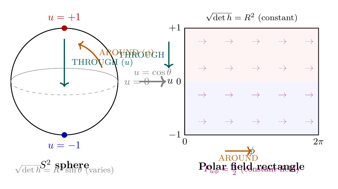
Throughout this book, \(S^2\) geometry is expressed in two equivalent coordinate systems. The spherical coordinates \((\theta, \phi)\) are the standard angular variables; the polar field coordinates \((u, \phi)\) use the substitution
Scaffolding note: The polar field variable \(u = \cos\theta\) is a coordinate choice, not a new physical assumption. Every result derived in polar coordinates is identically obtainable in spherical coordinates. The polar form is preferred throughout this book because it makes the flat integration measure, constant field strength, and around/through decomposition manifest.
Polar Metric and Determinant
In polar field coordinates \((u, \phi)\), the round metric on \(S^2\) of radius \(R\) takes the form
The metric determinant in polar field coordinates is constant:
Integration Measure
Because \(\sqrt{\det h} = R^2\) is constant, the natural integration measure on \(S^2\) in polar field coordinates is the flat Lebesgue measure:
Monopole Connection and Field Strength
The monopole field strength in polar coordinates is
Monopole Harmonics
The fundamental monopole harmonics (\(j = 1/2\), charge \(q = 1/2\)) have squared amplitudes that are linear in \(u\):
Around/Through Decomposition
In polar field coordinates, the two directions on \(S^2\) acquire distinct physical identities:
Polar Laplacian
The Laplacian on \(S^2\) in polar field coordinates takes the Legendre form:
Comparison Table: Spherical vs Polar Notation
Quantity | Spherical \((\theta, \phi)\) | Polar field \((u, \phi)\) |
|---|---|---|
| Variable | \(\theta \in [0, \pi]\) | \(u = \cos\theta \in [-1, +1]\) |
| Metric determinant | \(\sqrt{\det h} = R^2\sin\theta\) (varies) | \(\sqrt{\det h} = R^2\) (constant) |
| Integration measure | \(\sin\theta\,d\theta\,d\phi\) | \(du\,d\phi\) (flat) |
| Connection | \(A_\phi = \frac{1}{2}(1-\cos\theta)\) | \(A_\phi = \frac{1}{2}(1-u)\) (linear) |
| Field strength | \(F_{\theta\phi} = \frac{1}{2}\sin\theta\) | \(F_{u\phi} = \frac{1}{2}\) (constant) |
| \(|Y_+|^2\) | \(\cos^2(\theta/2)/(2\pi)\) | \((1+u)/(4\pi)\) (linear) |
| Laplacian eigenfunctions | \(Y_{\ell m}(\theta,\phi)\) (trig) | \(P_\ell^{|m|}(u)\,e^{im\phi}\) (polynomial) |
| Key integral | \(\int\sin^3\theta\,d\theta\) (trig) | \(\int(1-u^2)\,du = 4/3\) (polynomial) |
Key Polar Integrals
The following integrals appear repeatedly throughout the book:
Index Conventions and Summation Rules
4D Spacetime Indices
Greek indices \(\mu, \nu, \rho, \sigma, \ldots = 0, 1, 2, 3\) label spacetime coordinates in the four-dimensional continuum:
Spatial Indices — 3D Subspace
Latin indices \(i, j, k, \ell, \ldots = 1, 2, 3\) label the three spatial coordinates:
6D Scaffolding Indices
The \(S^2\) projection structure carries its own index pair:
When using polar field coordinates, the \(S^2\) indices \(i, j\) label the coordinates \((u, \phi)\) rather than \((\theta, \phi)\). The metric components become \(h_{uu} = R^2/(1-u^2)\), \(h_{\phi\phi} = R^2(1-u^2)\), and \(h_{u\phi} = 0\). Index raising and lowering follows the standard rule: \(V^u = h^{uu} V_u = [(1-u^2)/R^2]\,V_u\). All tensor equations are coordinate-invariant; the polar form is preferred because \(\sqrt{\det h} = R^2\) is constant. See Section app:e:polar-coords for the complete polar notation.
Capital indices \(A, B, C, \ldots = 0, 1, 2, 3, 4, 5\) (or \(0, 1, 2, 3, 5, 6\) in some conventions) label all six coordinates of the mathematical scaffolding:
Einstein Summation Convention
We employ the Einstein summation convention: any index appearing exactly twice in a monomial (once raised, once lowered) is summed over its full range:
Units and Physical Constants
Natural Units System
Throughout this work, we adopt natural units in which the reduced Planck constant and speed of light are set to unity:
To convert a result from natural units to SI units, one must restore \(\hbar\) and \(c\) using dimensional analysis. For example:
- An energy \(E\) in natural units is converted to SI by multiplication by a factors of \(c\): \([E]_{\text{SI}} = E \times c\) (adjusting dimensionally).
- The fundamental relation \([E] = \sqrt{[M][L]^{-1}}\) in natural units gives the correct dimensional form when \(\hbar\) and \(c\) are restored.
- Commonly used conversion factors:
Planck Mass and Planck Scale
The Planck mass is defined as
Key Physical Constants with Dimensions
The following fundamental parameters carry dimensions and appear throughout TMT:
The characteristic length scale appearing in TMT's derivations is
In the 6D scaffolding formalism, the 6D Planck mass is
Unit Systems Used
Context | Convention | Example |
|---|---|---|
| Theoretical derivations | Natural units: \(\hbar = c = 1\) | \([m] = [E]\); e.g., \(m = 0.511\,\text{MeV}\) |
| Particle physics phenomenology | Energy units (GeV, MeV) | Coupling: \(\alpha = 1/137\) (dimensionless) |
| Cosmology | Time \(t\), distance \(d\) in SI | \(H_0 = 73.3\,\km / \text{s} / \,\text{Mpc}\) |
| Quantum mechanics | \(\hbar\) restored explicitly | Energy-time: \(\Delta E \Delta t \geq \hbar/2\) |
| Gravity | \(G_N\) explicit | Planck mass: \(M_{\text{Pl}} = \sqrt{\hbar c/G_N}\) |
Spinor Conventions
A spinor is a section of the spinor bundle, which is a lift of the orthonormal frame bundle \(O(M)\) to the spin group Spin\((n)\). For a 4D Lorentzian manifold, the structure group is Spin\((1,3) \cong SL(2, \mathbb{C})\), which is the universal cover of the Lorentz group SO\((1,3)\).
A Dirac spinor \(\psi\) is a four-component complex vector transforming in the \((1/2, 0) \oplus (0, 1/2)\) representation of the Lorentz algebra:
Gamma Matrices and Clifford Algebra
The Dirac gamma matrices \(\gamma^\mu\) satisfy the Clifford algebra relation
The chiral projectors are
Weyl Spinors and Conjugation
A Weyl spinor is a two-component complex spinor transforming under a single irreducible representation of the Lorentz group. The left-handed Weyl spinor \(\xi_L\) and its right-handed counterpart \(\xi_R\) are related by:
The Dirac conjugate of a spinor \(\psi\) is
Field Definitions and Quantum Field Properties
Classical and Quantum Fields
A scalar field \(\phi(x)\) is a function assigning a complex number to each spacetime point \(x = (t, \mathbf{x})\):
A vector field (4-vector) \(V^\mu(x)\) assigns a 4-component vector to each spacetime point:
A spinor field \(\psi(x)\) assigns a Dirac spinor to each spacetime point:
Covariant Derivatives and Gauge Coupling
The covariant derivative of a field \(\Phi\) in a gauge theory with group \(G\) and coupling constant \(g\) is
For an abelian gauge group (e.g., \(U(1)_{\text{EM}}\)), the electromagnetic field strength is
The Higgs Doublet and Electroweak Symmetry
The Higgs field is a \(SU(2)_L\) doublet of complex scalars
The Yukawa coupling between the Higgs field and fermion doublets generates fermion masses. For a generic fermion \(f\),
Standard Model Field Content
Field | Type | \(SU(3)_c\) | \(SU(2)_L\) | \(U(1)_Y\) | Spin |
|---|---|---|---|---|---|
| Quark doublet \(Q_L\) | Fermi | \(\mathbf{3}\) | \(\mathbf{2}\) | \(1/6\) | \(1/2\) |
| Up quark \(u_R\) | Fermi | \(\mathbf{3}\) | \(\mathbf{1}\) | \(2/3\) | \(1/2\) |
| Down quark \(d_R\) | Fermi | \(\mathbf{3}\) | \(\mathbf{1}\) | \(-1/3\) | \(1/2\) |
| Lepton doublet \(L_L\) | Fermi | \(\mathbf{1}\) | \(\mathbf{2}\) | \(-1/2\) | \(1/2\) |
| Charged lepton \(e_R\) | Fermi | \(\mathbf{1}\) | \(\mathbf{1}\) | \(-1\) | \(1/2\) |
| Higgs doublet \(H\) | Scalar | \(\mathbf{1}\) | \(\mathbf{2}\) | \(1/2\) | \(0\) |
| Gluon \(g\) | Vector | \(\mathbf{8}\) | \(\mathbf{1}\) | \(0\) | \(1\) |
| \(W^\pm\), \(Z\) | Vector | \(\mathbf{1}\) | \(\mathbf{3}\) | \(0\) | \(1\) |
| Photon \(\gamma\) | Vector | \(\mathbf{1}\) | \(\mathbf{1}\) | \(0\) | \(1\) |
Dimensional Analysis and Scale Dependence
In natural units (\(\hbar = c = 1\)), every quantity has dimensions expressible as a power of mass \([M]\):
The running of coupling constants with energy scale is described by the renormalization group equation (RGE):
Coupling Constants and Interface Parameters
The fine structure constant governing electromagnetic interactions is
The weak interaction coupling constant \(g\) is related to the fine structure constant and the Weinberg angle \(\theta_W\) by
The strong interaction is characterized by the QCD coupling \(\alpha_s\), which runs with energy scale:
In the Temporal Momentum Theory framework, the interface between 4D physics and the \(S^2\) projection structure introduces a characteristic coupling strength
Polar Field Form of the Interface Coupling
In polar field coordinates, the interface coupling \(g^2 = 4/(3\pi)\) reduces to a single polynomial integral. The coupling arises from the \(S^2\) overlap of monopole harmonics:
Summary Table of Key Notation
Notation | Meaning | Value/Range |
|---|---|---|
| \multicolumn{3}{c}{Spacetime and Indices} | ||
| \(\mu, \nu\) | 4D spacetime indices | \(0, 1, 2, 3\) |
| \(i, j, k\) | Spatial indices (3D) | \(1, 2, 3\) |
| \(a, b\) | \(S^2\) projection indices | \(4, 5\) (or \(\theta, \phi\)) |
| \(A, B, C\) | Full 6D ambient indices | \(0, 1, 2, 3, 4, 5\) |
| \(g_{\mu\nu}\) | 4D metric (signature \(-+++\)) | Minkowski or curved |
| \(h_{ab}\) | \(S^2\) metric | Round metric on 2-sphere |
| \multicolumn{3}{c}{Constants and Scales} | ||
| \(\hbar, c\) | Planck constant, speed of light | \(\hbar = c = 1\) (natural units) |
| \(M_{\text{Pl}}\) | Planck mass (non-reduced) | \(1.221 \times 10^{19}\,\text{GeV}\) |
| \(\ell_{\text{Pl}}\) | Planck length | \(1.616 \times 10^{-35}\,\text{m}\) |
| \(v\) | Higgs VEV | \(246\,\text{GeV}\) |
| \(L_\mu\) | Interface scale | \(81\,\mu\text{m}\) |
| \(M_6\) | 6D Planck mass (scaffolding) | \(7296\,\text{GeV}\) |
| \(\alpha\) | Fine structure constant | \(1/137.036\) |
| \(\alpha_s(M_Z)\) | Strong coupling at \(Z\) mass | \(\approx 0.118\) |
| \multicolumn{3}{c}{Spinors and Fields} | ||
| \(\psi\) | Dirac spinor (4-component) | \(\mathbb{C}^4\) |
| \(\xi_L, \xi_R\) | Left/right Weyl spinors | \(\mathbb{C}^2\) each |
| \(\phi\) | Scalar field | \(\mathbb{C}\) at each point |
| \(A_\mu\) | Vector (gauge) field | \(\mathbb{R}^4\) at each point |
| \(\gamma^\mu\) | Dirac gamma matrices | Clifford algebra generators |
| \(P_L, P_R\) | Chiral projectors | \((1 \mp \gamma^5)/2\) |
| \multicolumn{3}{c}{Polar Field Coordinates on \(S^2\)} | ||
| \(u = \cos\theta\) | Polar field variable | \(u \in [-1, +1]\) |
| \(du\,d\phi\) | Flat integration measure | Constant \(\sqrt{\det h} = R^2\) |
| \(F_{u\phi} = 1/2\) | Monopole field strength | Constant (no \(\sin\theta\)) |
| \(A_\phi = (1-u)/2\) | Monopole connection | Linear in \(u\) |
| \(|Y_\pm|^2\) | Monopole harmonic densities | \((1\pm u)/(4\pi)\) (linear) |
| THROUGH (\(u\)) | Polar direction | Mass, gravity |
| AROUND (\(\phi\)) | Azimuthal direction | Gauge, charge |
| \(\langle u^2\rangle = 1/3\) | Second moment | Origin of factor 3 |
| \multicolumn{3}{c}{6D Scaffolding (Mathematical, Not Physical)} | ||
| \(ds_6^{\,2}\) | 6D metric interval | \(= 0\) (P1 postulate) |
| \(S^2\) | 2-sphere projection structure | Embedded in formalism |
| \(\mathcal{M}^4 \times S^2\) | Product manifold (math arena) | Not physical extra dimensions |
Derived Units and Common Conversions
When working between natural units and SI/CGS, the following conversions are useful:
Notation for Calculus and Linear Algebra
For a matrix \(M\),
Conclusion: Consistency and Self-Reference
The conventions established in this appendix provide a complete, self-consistent framework for interpreting all equations, theorems, and results throughout this book. Key principles:
- Metric signature \((-+++)\) is universal: All spacetime calculations employ this convention.
- Natural units (\(\hbar = c = 1\)) are default: Factors are restored where clarity demands.
- 6D formalism is scaffolding, not ontology: The mathematics is 6D; the physics is 4D.
- All constants carry dimensions: This prevents unit-system errors and clarifies physical meaning.
- Index conventions are rigid: Greek indices for 4D spacetime, Latin for spatial components, capital for 6D. Violations are flagged as errors.
- Spinor conventions follow QFT standard: Dirac spinors with chiral projectors, Weyl representation gamma matrices.
- Polar field coordinates are canonical on \(S^2\): The substitution \(u = \cos\theta\) yields a flat integration measure \(du\,d\phi\) with constant metric determinant \(\sqrt{\det h} = R^2\). All \(S^2\) integrals become polynomial integrals on \([-1,+1]\), and the around/through decomposition becomes literal in these coordinates.
This appendix serves as the definitive reference for any notation ambiguity encountered elsewhere in the book.
Derivation Chain Summary
# | Step | Justification | Reference |
|---|---|---|---|
| \endhead 1 | Metric signature \((-+++)\) | Standard Lorentzian convention | \Sapp:e:metric-signature |
| 2 | Natural units \(\hbar = c = 1\) | Dimensional analysis | \Sapp:e:units-constants |
| 3 | 6D scaffolding structure | Block-diagonal \(g_{\mu\nu} \oplus h_{ij}\) | \Sapp:e:metric-signature |
| 4 | Index conventions | \(\mu\nu\) (4D), \(ij\) (spatial), \(AB\) (6D), \(ab\) (\(S^2\)) | \Sapp:e:indices |
| 5 | Spinor and field conventions | Chiral basis, Clifford algebra, gauge coupling | \Sapp:e:spinor-conventions–app:e:field-definitions |
| 6 | Polar: \(u = \cos\theta\) on \(S^2\) | Coordinate substitution; \(\sqrt{\det h} = R^2\) constant, \(du\,d\phi\) flat, \(F_{u\phi} = 1/2\) constant, \(|Y_\pm|^2 = (1\pm u)/(4\pi)\) linear | \Sapp:e:polar-coords |