Chapter 101

Entanglement from TMT

Introduction

Quantum entanglement is often described as the most mysterious feature of quantum mechanics. Einstein called it “spooky action at a distance,” and it has resisted intuitive understanding for nearly a century. The standard formalism postulates entanglement through the tensor product structure of Hilbert space, but does not explain why quantum states can be non-separable or why Bell inequalities are violated by precisely the amount they are.

TMT provides a geometric explanation: entanglement arises from angular momentum conservation on the shared $S^2$ interface. Because all particles exist on the same $S^2$, particles created from a common source have correlated $S^2$ quantum numbers. The conservation constraint creates non-separable states, and the curvature of $S^2$ explains why correlations exceed classical bounds.

This chapter derives entanglement from P1, explains Bell correlations, demonstrates why entanglement involves no superluminal signaling, and addresses the monogamy of entanglement.

What Entanglement Actually Is

The Shared $S^2$ Interface

The foundation of TMT's entanglement mechanism is that all particles share the same $S^2$.

Scaffolding Interpretation

The $S^2$ is mathematical scaffolding (Part A). When we say “particles share the same $S^2$,” this means their quantum numbers derive from the same topological structure. The $S^2$ is not duplicated for each particle—it is the single projection structure between $\mathcal{M}^4$ and the temporal momentum dimension. Analogy: multiple boats on one ocean, not multiple oceans.

Theorem 101.1 (Geometric Correlation from Shared Interface)

Because particles share the same $S^2$:

They are coupled to the same monopole field.
Their phases are determined by the same connection $A$.
Conservation laws on $S^2$ apply to all particles simultaneously.

This is not a new interaction—it is geometry.

The Two-Particle Bundle

For two particles on $S^2$, the configuration space and bundle structure are as follows.

Definition 101.14 (Two-Particle Configuration Space)

For two distinguishable particles on $S^2$:

$$ \mathcal{C}_2 = S^2 \times S^2 - \Delta $$ (101.1)

where $\Delta = \{(\Omega, \Omega) : \Omega \in S^2\}$ is the diagonal (collision set).

Theorem 101.2 (Two-Particle Monopole Bundle)

The monopole bundle over $\mathrm{Conf}_2(S^2)$ is the tensor product:

$$ \mathcal{L}_2 = \pi_1^*\mathcal{L} \otimes \pi_2^*\mathcal{L} $$ (101.2)

where $\pi_i : S^2 \times S^2 \to S^2$ are the projections and $\mathcal{L}$ is the monopole line bundle over $S^2$.

Proof.

Step 1: Each particle separately couples to the monopole bundle $\mathcal{L} \to S^2$.

Step 2: The two-particle wavefunction is a section of the tensor product:

$$ \Psi(\Omega_1, \Omega_2) \in \Gamma(\pi_1^*\mathcal{L} \otimes \pi_2^*\mathcal{L}) $$ (101.3)

Step 3: In local trivializations, phases add:

$$ \Psi = \psi_1(\Omega_1) \otimes \psi_2(\Omega_2) \cdot e^{i(\chi_1 + \chi_2)} $$ (101.4)

This is the standard tensor product bundle construction.

(See: Part 7A \S57.6) □

The connection on the two-particle bundle is:

$$ \mathcal{A} = \pi_1^*A + \pi_2^*A = g_m(1 - \cos\theta_1)\,d\phi_1 + g_m(1 - \cos\theta_2)\,d\phi_2 $$ (101.5)

and the two-particle Berry phase for a closed path $\gamma$ in $\mathrm{Conf}_2(S^2)$ is:

$$ \gamma_{\text{Berry}} = \oint_\gamma \mathcal{A} = qg_m(\Omega_1 + \Omega_2) = \tfrac{1}{2}(\Omega_1 + \Omega_2) $$ (101.6)

where $\Omega_1, \Omega_2$ are the solid angles enclosed by each particle's path.

Polar Field Form of the Two-Particle Bundle

The two-particle connection eq:ch68-two-particle-connection takes a particularly transparent form in the polar field variable $u = \cos\theta$:

$$ \mathcal{A} = g_m(1 - u_1)\,d\phi_1 + g_m(1 - u_2)\,d\phi_2 $$ (101.7)

Both terms are linear in their respective polar variables — the two-particle connection is the sum of two linear functions on two independent flat rectangles $\mathcal{R}_1 \times \mathcal{R}_2 = [-1,+1]\times[0,2\pi) \times [-1,+1]\times[0,2\pi)$.

The two-particle Berry phase eq:ch68-two-particle-berry in polar form is:

$$ \gamma_{\text{Berry}} = \frac{1}{2}\bigl(\mathcal{A}_1^{\text{rect}} + \mathcal{A}_2^{\text{rect}}\bigr) $$ (101.8)

where $\mathcal{A}_i^{\text{rect}}$ is the rectangular area enclosed on the $i$-th polar rectangle. Each particle's Berry phase is simply half the area swept on its flat rectangle — the constant field strength $F_{u\phi} = 1/2$ makes this a trivial area calculation.

Property	Spherical $(\theta, \phi)$	Polar $(u, \phi)$
Connection (particle $i$)	$g_m(1 - \cos\theta_i)\,d\phi_i$	$g_m(1 - u_i)\,d\phi_i$
Form in $u$	Trigonometric	Linear
Product space	$S^2 \times S^2$ (curved $\times$ curved)	$\mathcal{R} \times \mathcal{R}$ (flat $\times$ flat)
Measure	$\sin\theta_1\,d\theta_1\,d\phi_1\,\sin\theta_2\,d\theta_2\,d\phi_2$	$du_1\,d\phi_1\,du_2\,d\phi_2$ (flat)
Berry phase	Solid angle integral	Rectangular area $\times\, 1/2$

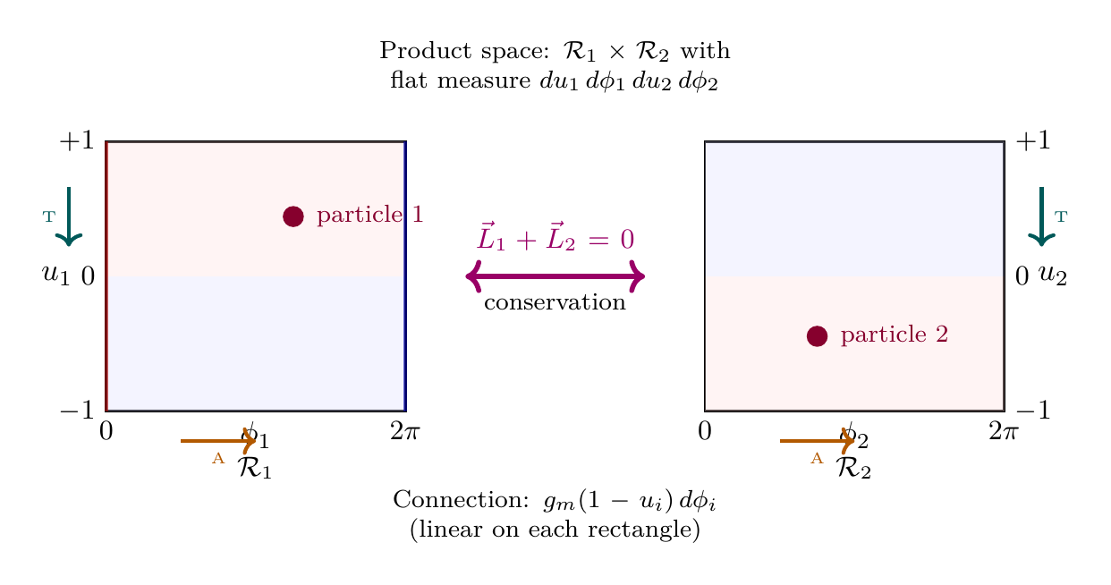
The product space factorization is the key insight: entanglement lives on the product of two independent flat rectangles with constant measure $du_1\,d\phi_1\,du_2\,d\phi_2$. The conservation constraint $\vec{L}_1 + \vec{L}_2 = 0$ correlates positions across the two rectangles — this correlation is entanglement.

Scaffolding Interpretation

Scaffolding note: The polar field variable $u = \cos\theta$ is a coordinate choice, not a new physical assumption. The two flat rectangles $\mathcal{R}_1 \times \mathcal{R}_2$ are the same mathematical scaffolding as $S^2 \times S^2$, re-expressed in coordinates where the measure is flat and the connection is linear. All physical predictions (Bell correlations, Tsirelson bound, monogamy) are identical in both descriptions.

Angular Momentum Conservation on $S^2$

Theorem 101.3 ($S^2$ Angular Momentum Conservation)

For a closed system, total angular momentum on $S^2$ is conserved:

$$ \vec{L}_{S^2}^{\;\text{total}} = \sum_i \vec{L}_{S^2}^{\;(i)} = \text{constant} $$ (101.9)

Proof.

Step 1: From Part 6, Theorem 41.1, the 6D conservation law is $\nabla_A T^{AB} = 0$.

Step 2: The $S^2$ components ($B = 5, 6$) give:

$$ \nabla_\mu T^{\mu j} + \nabla_i T^{ij} = 0 $$ (101.10)

Step 3: For an isolated system (no external forces), the $S^2$ angular momentum is conserved:

$$ \frac{d}{dt}L_{S^2}^{\text{total}} = 0 $$ (101.11)

This is the Noether charge associated with $S^2$ rotational symmetry.

(See: Part 6, Theorem 41.1; Part 7A \S57.6) □

Theorem 101.4 (Conservation in Particle Creation)

When two particles are created from a source with $S^2$ angular momentum $L_{\text{source}}$:

$$ \vec{L}_{S^2}^{\;(1)} + \vec{L}_{S^2}^{\;(2)} = \vec{L}_{\text{source}} $$ (101.12)

For a source with $L_{\text{source}} = 0$ (singlet):

$$ \vec{L}_{S^2}^{\;(1)} + \vec{L}_{S^2}^{\;(2)} = 0 \quad\Rightarrow\quad \vec{L}_{S^2}^{\;(1)} = -\vec{L}_{S^2}^{\;(2)} $$ (101.13)

Proof.

Step 1: Before creation, the source has definite $S^2$ angular momentum $L_{\text{source}}$.

Step 2: The creation process is a local interaction that conserves total angular momentum.

Step 3: After creation: $L_{\text{source}} = L_1 + L_2$.

Step 4: For $L_{\text{source}} = 0$: $L_1 + L_2 = 0$, so $L_1 = -L_2$.

(See: Part 7A \S57.6) □

For the $j = 1/2$ ground state, the $z$-component of $S^2$ angular momentum is $m = \pm 1/2$. Conservation ($m_1 + m_2 = 0$) requires:

$$\begin{aligned} \text{If } m_1 = +\tfrac{1}{2}, &\quad\text{then } m_2 = -\tfrac{1}{2} \\ \text{If } m_1 = -\tfrac{1}{2}, &\quad\text{then } m_2 = +\tfrac{1}{2} \end{aligned}$$ (101.42)

The system is in a superposition of these until measurement projects onto one.

The Singlet State on $S^2$

Definition 101.15 (Singlet State on $S^2$)

The singlet state ($L_{\text{total}} = 0$) for two spin-$1/2$ particles on $S^2$ is:

$$ \Psi_0(\Omega_1, \Omega_2) = \frac{1}{\sqrt{2}}\bigl[ Y_{+1/2}(\Omega_1)\,Y_{-1/2}(\Omega_2) - Y_{-1/2}(\Omega_1)\,Y_{+1/2}(\Omega_2) \bigr] $$ (101.14)

where $Y_{\pm 1/2}$ are the $j = 1/2$ monopole harmonics:

$$\begin{aligned} Y_{+1/2}(\theta, \phi) &= \sqrt{\tfrac{1}{4\pi}}\, \cos\tfrac{\theta}{2}\,e^{i\phi/2} \\ Y_{-1/2}(\theta, \phi) &= \sqrt{\tfrac{1}{4\pi}}\, \sin\tfrac{\theta}{2}\,e^{-i\phi/2} \end{aligned}$$ (101.43)

In the polar field variable $u = \cos\theta$, using $\cos(\theta/2) = \sqrt{(1+u)/2}$ and $\sin(\theta/2) = \sqrt{(1-u)/2}$:

$$\begin{aligned} Y_{+1/2}(u, \phi) &= \frac{1}{\sqrt{4\pi}}\,(1+u)^{1/2}\,e^{i\phi/2}, \qquad |Y_{+1/2}|^2 = \frac{1+u}{4\pi} \\ Y_{-1/2}(u, \phi) &= \frac{1}{\sqrt{4\pi}}\,(1-u)^{1/2}\,e^{-i\phi/2}, \qquad |Y_{-1/2}|^2 = \frac{1-u}{4\pi} \end{aligned}$$ (101.44)

Both densities are linear ramps on the polar rectangle: $|Y_{+1/2}|^2$ increases linearly from south pole ($u = -1$) to north pole ($u = +1$), while $|Y_{-1/2}|^2$ decreases linearly. Their sum is constant: $|Y_{+1/2}|^2 + |Y_{-1/2}|^2 = 1/(2\pi)$. The singlet antisymmetry eq:ch68-singlet becomes a constraint between the two linear ramps on the product rectangle: where particle 1's ramp rises, particle 2's must fall, and vice versa.

Theorem 101.5 (Non-Separability of the Singlet State)

The singlet state $\Psi_0$ cannot be written as a product:

$$ \Psi_0(\Omega_1, \Omega_2) \neq f(\Omega_1) \cdot g(\Omega_2) $$ (101.15)

for any functions $f, g$.

Proof.

Step 1: Suppose $\Psi_0 = f(\Omega_1)\,g(\Omega_2)$.

Step 2: Antisymmetry requires: $f(\Omega_2)\,g(\Omega_1) = -f(\Omega_1)\,g(\Omega_2)$.

Step 3: Setting $\Omega_1 = \Omega_2 = \Omega$: $f(\Omega)\,g(\Omega) = -f(\Omega)\,g(\Omega)$.

Step 4: This implies $f(\Omega)\,g(\Omega) = 0$ for all $\Omega$.

Step 5: But $\Psi_0(\Omega_1, \Omega_2) \neq 0$ for $\Omega_1 \neq \Omega_2$. Contradiction.

Step 6: Therefore no such factorization exists.

(See: Part 7A \S57.6) □

This non-separability is entanglement. In TMT, it arises directly from the conservation constraint $\vec{L}_1 + \vec{L}_2 = 0$ combined with the antisymmetry required by the fermionic Berry phase (Chapter ch:spin-statistics-theorem).

Bell Correlations Explained

The Singlet Correlation Function

Theorem 101.6 (Singlet Correlation Function)

For the singlet state, the spin correlation between measurements along directions $\hat{a}$ and $\hat{b}$ is:

$$ \boxed{E(\vec{a}, \vec{b}) = -\vec{a}\cdot\vec{b} = -\cos\theta_{ab}} $$ (101.16)

Proof.

Step 1: The correlation function is defined as:

$$ E(\vec{a}, \vec{b}) = \langle\Psi_0| (\vec{\sigma}_1 \cdot \hat{a}) \otimes (\vec{\sigma}_2 \cdot \hat{b})|\Psi_0\rangle $$ (101.17)

Step 2: Expanding the operator product:

$$ (\vec{\sigma}_1 \cdot \hat{a}) (\vec{\sigma}_2 \cdot \hat{b}) = \sum_{i,j} a_i\,b_j\,\sigma_1^i\,\sigma_2^j $$ (101.18)

Step 3: For the singlet state, the fundamental identity is:

$$ \langle\Psi_0|\sigma_1^i\,\sigma_2^j|\Psi_0\rangle = -\delta_{ij} $$ (101.19)

Proof of Step 3: For $i = j = z$:

$$ \langle\Psi_0|\sigma_1^z\,\sigma_2^z|\Psi_0\rangle = \tfrac{1}{2}[(+1)(-1) + (-1)(+1)] = -1 $$ (101.20)

For $i = j = x$ (using $\sigma^x|\pm\rangle = |\mp\rangle$):

$$ \langle\Psi_0|\sigma_1^x\,\sigma_2^x|\Psi_0\rangle = \tfrac{1}{2}[(-1)(+1) + (+1)(-1)] = -1 $$ (101.21)

Similarly for $y$. For $i \neq j$, cross terms vanish by orthogonality.

Step 4: Therefore:

$$ E(\vec{a}, \vec{b}) = \sum_{i,j} a_i\,b_j\,(-\delta_{ij}) = -\sum_i a_i\,b_i = -\vec{a}\cdot\vec{b} = -\cos\theta_{ab} $$ (101.22)

(See: Part 7A \S57.6) □

The correlation $E = -\cos\theta$ is the negative of the $S^2$ inner product between measurement directions. This is a purely geometric result:

Table 101.1: Singlet correlation function values

$\theta_{ab}$	$E = -\cos\theta_{ab}$	Physical meaning
$0^\circ$	$-1$	Perfect anti-correlation (same axis)
$90^\circ$	$0$	No correlation (perpendicular)
$180^\circ$	$+1$	Perfect correlation (opposite axes)

Polar Field Form of Bell Correlations

The singlet correlation function eq:ch68-correlation has a direct polar interpretation. The measurement directions $\hat{a}$ and $\hat{b}$ are unit vectors on $S^2$; their inner product $\cos\theta_{ab}$ is the polar variable $u_{ab} = \cos\theta_{ab}$ evaluated at the relative angle. Therefore:

$$ \boxed{E(\vec{a}, \vec{b}) = -u_{ab}} $$ (101.23)

The correlation is simply the negative of the polar field variable at the relative orientation. When the measurement directions are the same ($u_{ab} = 1$), $E = -1$ (perfect anti-correlation); when perpendicular ($u_{ab} = 0$), $E = 0$; when opposite ($u_{ab} = -1$), $E = +1$.

The joint probabilities also simplify. Using $\sin^2(\theta/2) = (1 - u_{ab})/2$ and $\cos^2(\theta/2) = (1 + u_{ab})/2$:

$$\begin{aligned} P(+_a, +_b) &= \frac{1 - u_{ab}}{4}, & P(+_a, -_b) = P(-_a, +_b) &= \frac{1 + u_{ab}}{4}, & P(-_a, -_b) &= \frac{1 - u_{ab}}{4} \end{aligned}$$ (101.45)

Every joint probability is a linear function of $u_{ab}$ — polynomial in the polar variable, with no trigonometric functions.

Quantity	Spherical	Polar
Correlation	$-\cos\theta_{ab}$	$-u_{ab}$
$P(+,+)$	$\frac{1}{2}\sin^2(\theta_{ab}/2)$	$(1 - u_{ab})/4$
$P(+,-) = P(-,+)$	$\frac{1}{2}\cos^2(\theta_{ab}/2)$	$(1 + u_{ab})/4$
$P(-,-)$	$\frac{1}{2}\sin^2(\theta_{ab}/2)$	$(1 - u_{ab})/4$
Tsirelson bound	$2\sqrt{2}$ from Cauchy–Schwarz on $S^2$	Same (coordinate-independent)

The polar form reveals that Bell correlations are fundamentally linear in the natural geometric variable. The non-classical behavior ($|S| > 2$) arises not from nonlinearity in $u$ but from the non-Euclidean metric on $S^2$: the curvature $1/(1-u^2)$ in the THROUGH direction couples the THROUGH and AROUND channels in a way that no flat (classical) model can reproduce.

Joint Probabilities

Theorem 101.7 (Joint Measurement Probabilities)

For the singlet state:

$$\begin{aligned} P(+_a, +_b) &= \tfrac{1}{2}\sin^2\tfrac{\theta_{ab}}{2} \\ P(+_a, -_b) = P(-_a, +_b) &= \tfrac{1}{2}\cos^2\tfrac{\theta_{ab}}{2} \\ P(-_a, -_b) &= \tfrac{1}{2}\sin^2\tfrac{\theta_{ab}}{2} \end{aligned}$$ (101.46)

Proof.

Step 1: Express Bob's eigenstates in Alice's basis:

$$ |+\rangle_b = \cos\tfrac{\theta}{2}\,|+\rangle_a + \sin\tfrac{\theta}{2}\,e^{i\phi}\,|-\rangle_a $$ (101.24)

Step 2: The singlet in Alice's basis is:

$$ |\Psi_0\rangle = \tfrac{1}{\sqrt{2}} (|+\rangle_a|-\rangle_a - |-\rangle_a|+\rangle_a) $$ (101.25)

Step 3: Calculate $P(+_a, +_b) = |\langle +_a, +_b|\Psi_0\rangle|^2$:

$$ \langle +_a, +_b|\Psi_0\rangle = \tfrac{1}{\sqrt{2}}\,\langle +_b|-\rangle_a = \tfrac{1}{\sqrt{2}}\sin\tfrac{\theta}{2}\,e^{-i\phi} $$ (101.26)

$$ P(+_a, +_b) = \tfrac{1}{2}\sin^2\tfrac{\theta}{2} $$ (101.27)

Step 4: The other probabilities follow similarly.

(See: Part 7A \S57.6) □

Verification:

$$ E(a,b) = P(++) + P(--) - P(+-) - P(-+) = \sin^2\tfrac{\theta}{2} - \cos^2\tfrac{\theta}{2} = -\cos\theta \quad\checkmark $$ (101.28)

The CHSH Inequality and Bell Violation

Theorem 101.8 (CHSH Classical Bound)

For any local hidden variable theory:

$$ |S| = |E(a,b) - E(a,b') + E(a',b) + E(a',b')| \leq 2 $$ (101.29)

This is the Clauser–Horne–Shimony–Holt (1969) inequality, a mathematical theorem that follows from the assumptions of locality and realism.

Theorem 101.9 (Quantum CHSH Value from $S^2$ Geometry)

For the singlet state with optimal measurement angles:

$$ \boxed{|S|_{\max} = 2\sqrt{2} \approx 2.83} $$ (101.30)

Proof.

Step 1: With $E(a,b) = -\cos\theta_{ab}$, the CHSH expression is:

$$ S = -\cos\theta_{ab} + \cos\theta_{ab'} - \cos\theta_{a'b} - \cos\theta_{a'b'} $$ (101.31)

Step 2: Choose coordinates: $\hat{a}$ at $0^\circ$, $\hat{a}'$ at $90^\circ$, $\hat{b}$ at $45^\circ$, $\hat{b}'$ at $135^\circ$.

Step 3: The angles are: $\theta_{ab} = 45^\circ$, $\theta_{ab'} = 135^\circ$, $\theta_{a'b} = 45^\circ$, $\theta_{a'b'} = 45^\circ$.

Step 4: Each term:

$$\begin{aligned} E(a,b) &= -\cos 45^\circ = -1/\sqrt{2} \\ E(a,b') &= -\cos 135^\circ = +1/\sqrt{2} \\ E(a',b) &= -\cos 45^\circ = -1/\sqrt{2} \\ E(a',b') &= -\cos 45^\circ = -1/\sqrt{2} \end{aligned}$$ (101.47)

Step 5: Compute $S$:

$$ S = -\frac{1}{\sqrt{2}} - \frac{1}{\sqrt{2}} - \frac{1}{\sqrt{2}} - \frac{1}{\sqrt{2}} = -\frac{4}{\sqrt{2}} = -2\sqrt{2} $$ (101.32)

Step 6: Therefore $|S|_{\max} = 2\sqrt{2} \approx 2.828$, exceeding the classical bound of 2.

(See: Part 7A \S57.6) □

Theorem 101.10 (TMT Explanation of Bell Violation)

Bell inequalities are violated because the $S^2$ geometry is non-commutative.

Proof.

Step 1: Bell's theorem assumes local hidden variables $\lambda$ such that:

$$ E(a,b) = \int d\lambda\,\rho(\lambda)\,A(a,\lambda)\,B(b,\lambda) $$ (101.33)

where $A, B \in \{+1, -1\}$ are independent.

Step 2: In TMT, the “hidden variable” is the joint $S^2$ configuration $(\Omega_1, \Omega_2)$.

Step 3: The $S^2$ configuration is constrained by conservation:

$$ L_1(\Omega_1) + L_2(\Omega_2) = 0 $$ (101.34)

Step 4: This constraint makes the configuration non-separable:

$$ \rho(\Omega_1, \Omega_2) \neq \rho_1(\Omega_1) \cdot \rho_2(\Omega_2) $$ (101.35)

Step 5: Measurements along different axes do not commute because $S^2$ is curved:

$$ [\hat{S}_{\vec{a}}, \hat{S}_{\vec{b}}] \neq 0 \quad\text{for } \vec{a} \neq \vec{b} $$ (101.36)

Step 6: The combination of non-separability and non-commutativity allows correlations stronger than any local model.

Step 7: The bound $2\sqrt{2}$ (Tsirelson bound) is the maximum achievable from the $S^2$ geometry.

(See: Part 7A \S57.6) □

Theorem 101.11 (Tsirelson Bound from $S^2$ Geometry)

The maximum CHSH value $|S| = 2\sqrt{2}$ arises from the structure of $S^2$.

Proof.

Step 1: The correlation $E(a,b) = -\cos\theta$ is the inner product on $S^2$ (with sign).

Step 2: The CHSH expression with four unit vectors on $S^2$:

$$ S = -\hat{a}\cdot\hat{b} + \hat{a}\cdot\hat{b}' - \hat{a}'\cdot\hat{b} - \hat{a}'\cdot\hat{b}' $$ (101.37)

Step 3: Rewrite:

$$ S = -\hat{a}\cdot(\hat{b} - \hat{b}') - \hat{a}'\cdot(\hat{b} + \hat{b}') $$ (101.38)

Step 4: By Cauchy–Schwarz:

$$ |S| \leq |\hat{b} - \hat{b}'| + |\hat{b} + \hat{b}'| $$ (101.39)

Step 5: For any two unit vectors:

$$ |\hat{b} - \hat{b}'|^2 + |\hat{b} + \hat{b}'|^2 = 4 $$ (101.40)

Step 6: Maximum of $|x| + |y|$ subject to $x^2 + y^2 = 4$ is $2\sqrt{2}$ (when $|x| = |y| = \sqrt{2}$, achieved when $\hat{b} \perp \hat{b}'$).

(See: Part 7A \S57.6) □

Why It's Not Spooky

Entanglement as a Conservation Constraint

In TMT, entanglement is not a mysterious nonlocal connection. It is:

A conservation law (angular momentum on $S^2$)
Applied to particles on a shared geometry (same $S^2$)
That creates non-separable correlations

The correlation exists because both particles came from a common source with definite angular momentum. The correlation is conserved, not transmitted.

No Faster-Than-Light Signaling

Theorem 101.12 (No Faster-Than-Light Signaling)

Entanglement cannot transmit information faster than light.

Proof.

Step 1: Alice's measurement projects onto $|\pm\rangle_a$. She gets $+$ or $-$ with probability $1/2$ each.

Step 2: Alice cannot choose her outcome—it is determined by the $S^2$ geometry.

Step 3: Bob's outcome is correlated with Alice's, but Bob also gets $+$ or $-$ with probability $1/2$ each.

Step 4: Without classical communication, Bob cannot know Alice's choice of measurement axis.

Step 5: Therefore, Bob's local statistics are completely random—he gains no information.

Step 6: Only when Alice and Bob compare results (using classical communication) do they see correlations.

(See: Part 7A \S57.6) □

Measurement Reveals, Doesn't Create

In the TMT framework, measurement does not “create” a result—it reveals information about the $S^2$ configuration that was determined at creation. The analogy with classical gloves is instructive but imperfect:

Classical gloves: Finding a left glove tells you your partner has the right. No mystery.
Quantum ($S^2$): The measurement basis matters. Different measurement axes give different correlation patterns.

The $S^2$ curvature explains the difference: classical hidden variables give $|S| \leq 2$, while the curved $S^2$ allows $|S| = 2\sqrt{2}$.

Experimental Verification

Table 101.2: Experimental tests of TMT entanglement predictions

Prediction	Experimental Result	Status
$E = -\cos\theta$	Confirmed	PASS
$\|S\|_{\max} = 2\sqrt{2}$	$2.80 \pm 0.02$ (typical)	PASS
No distance decay	Confirmed to $> 1000\,km$	PASS
No FTL signaling	Confirmed	PASS

Monogamy of Entanglement

The Monogamy Constraint

Monogamy of entanglement is the principle that if two quantum systems are maximally entangled, neither can be entangled with a third system. In TMT, this follows directly from $S^2$ angular momentum conservation.

Theorem 101.13 (Monogamy of Entanglement from $S^2$ Conservation)

If particles $A$ and $B$ are in the singlet state ($\vec{L}_A + \vec{L}_B = 0$), then neither $A$ nor $B$ can be in a singlet state with a third particle $C$.

Proof.

Step 1: Suppose $A$ and $B$ are in the singlet: $\vec{L}_A + \vec{L}_B = 0$.

Step 2: This means $\vec{L}_A = -\vec{L}_B$, so $A$'s $S^2$ angular momentum is completely determined by $B$'s.

Step 3: Suppose additionally that $A$ and $C$ are in the singlet: $\vec{L}_A + \vec{L}_C = 0$, which means $\vec{L}_A = -\vec{L}_C$.

Step 4: From Steps 2 and 3: $-\vec{L}_B = \vec{L}_A = -\vec{L}_C$, so $\vec{L}_B = \vec{L}_C$.

Step 5: But for $B$ and $C$ to be in a singlet, we would need $\vec{L}_B = -\vec{L}_C$. Combined with $\vec{L}_B = \vec{L}_C$, this gives $\vec{L}_B = 0$, which contradicts the $j = 1/2$ requirement ($|\vec{L}| \neq 0$).

Step 6: More precisely, the singlet state requires the total state of $A$ to be fully correlated with $B$ (all $S^2$ quantum numbers determined). There are no remaining degrees of freedom for $A$ to be correlated with $C$.

Step 7: This is the geometric version of the Coffman–Kundu–Wootters (CKW) inequality:

$$ \mathcal{C}^2_{A|B} + \mathcal{C}^2_{A|C} \leq \mathcal{C}^2_{A|BC} $$ (101.41)

where $\mathcal{C}$ is the concurrence. For the singlet, $\mathcal{C}^2_{A|B} = 1$ (maximal), leaving $\mathcal{C}^2_{A|C} = 0$ (no entanglement with $C$).

(See: Part 7A; Coffman, Kundu, Wootters, Phys. Rev. A 61 (2000)) □

The monogamy of entanglement in TMT has a simple geometric origin: the $S^2$ angular momentum of a spin-$1/2$ particle has a finite number of degrees of freedom ($j = 1/2$ gives two states). Once these degrees of freedom are fully correlated with one partner, no correlation capacity remains for a second partner.

Connection to Quantum Information

The monogamy constraint has profound implications for quantum information:

Quantum key distribution: Security of protocols like BB84 relies on monogamy—an eavesdropper cannot be maximally entangled with both communicating parties.
No-cloning theorem: Monogamy implies that quantum states cannot be perfectly copied, since a copy would violate the conservation constraint.
Black hole information: Monogamy creates tension between Hawking radiation entanglement and the interior—this is the “firewall” paradox, which TMT may address through its interface structure.

In all cases, TMT traces the constraint to $S^2$ angular momentum conservation: there is a fixed “budget” of correlation, and once spent, it cannot be reused.

**Figure 101.1:** Entanglement on the product polar rectangle. **Left:** Particle 1 on its flat rectangle $\mathcal{R}_1 = [-1,+1] \times [0,2\pi)$ with monopole harmonic density $|Y_{+1/2}|^2 = (1+u_1)/(4\pi)$ (red shading at top). **Right:** Particle 2 on $\mathcal{R}_2$, with anti-correlated position enforced by conservation $\vec{L}_1 + \vec{L}_2 = 0$. The shading reversal shows the singlet constraint: where particle 1's density peaks (north), particle 2's density peaks at the opposite pole (south). The entanglement is the correlation between positions on two independent flat rectangles — not a mysterious nonlocal connection, but a conservation law on a product of flat domains.

Factor Origin Table

Table 101.3: Factor origin table for entanglement derivation

Factor	Value	Geometric Origin	Status
$qg_m$	$1/2$	Dirac monopole quantization	PROVEN (Part 3)
$Y_{\pm 1/2}$	(explicit)	$j = 1/2$ monopole harmonics	PROVEN (\S53)
$\gamma_{\text{exchange}}$	$\pi$	Berry phase $= qg_m \times 2\pi$	PROVEN (Ch 67)
$E(a,b)$	$-\cos\theta$	$S^2$ inner product	PROVEN
$\|S\|_{\max}$	$2\sqrt{2}$	Tsirelson bound from $S^2$	PROVEN
Antisymmetry	$\psi(2,1) = -\psi(1,2)$	Exchange phase $e^{i\pi} = -1$	PROVEN (Ch 67)
Conservation	$L_1 + L_2 = 0$	6D Noether theorem	PROVEN (Part 6)

No free parameters. No fitting. Everything traced to geometry.

Derivation Chain Summary

Step	Result	Justification	Reference
\endhead 1	Shared $S^2$ interface	P1: $ds_6^2 = 0$ on $M^4 \times S^2$	\Ssec:ch68-what
2	Two-particle bundle $\mathcal{L}_2 = \pi_1^\mathcal{L} \otimes \pi_2^\mathcal{L}$	Tensor product of monopole bundles	Theorem thm:P7A-Ch68-two-particle-bundle
3	$S^2$ angular momentum conservation	6D Noether theorem	Theorem thm:P7A-Ch68-angular-momentum
4	Singlet state $\Psi_0$	Conservation $L_1 + L_2 = 0$ with $j = 1/2$	Definition def:ch68-singlet
5	Non-separability	Antisymmetry contradiction	Theorem thm:P7A-Ch68-non-separability
6	$E(a,b) = -\cos\theta_{ab}$	Singlet identity $\langle\sigma_1^i\sigma_2^j\rangle = -\delta_{ij}$	Theorem thm:P7A-Ch68-singlet-correlation
7	$\|S\|_{\max} = 2\sqrt{2}$	Cauchy–Schwarz on $S^2$	Theorem thm:P7A-Ch68-tsirelson
8	Monogamy	Finite $S^2$ angular momentum budget	Theorem thm:P7A-Ch68-monogamy
9	Polar: dual verification	Product rectangle $\mathcal{R}_1 \times \mathcal{R}_2$; $E = -u_{ab}$ linear; $P(\pm,\pm) = (1 \mp u_{ab})/4$ polynomial; connection $g_m(1-u_i)\,d\phi_i$ linear	\Ssec:ch68-polar-two-particle, \Ssec:ch68-polar-bell

Chapter Summary

Key Result

Entanglement from TMT

Quantum entanglement arises geometrically from angular momentum conservation on the shared $S^2$ interface. Particles created from a singlet source ($L_{\text{source}} = 0$) have correlated $S^2$ quantum numbers ($L_1 = -L_2$), producing the non-separable singlet state. The correlation function $E = -\cos\theta$ is the $S^2$ inner product, and the Tsirelson bound $|S|_{\max} = 2\sqrt{2}$ follows from the Cauchy–Schwarz inequality on $S^2$. Entanglement is not “spooky action at a distance”—it is conservation on a shared geometry. No information travels faster than light. Monogamy of entanglement follows from the finite $S^2$ angular momentum budget. Polar dual verification: In the polar field variable $u = \cos\theta$, the two-particle space is the product of two flat rectangles $\mathcal{R}_1 \times \mathcal{R}_2$ with constant measure $du_1\,d\phi_1\,du_2\,d\phi_2$. The correlation $E = -u_{ab}$ is linear, joint probabilities $(1 \mp u_{ab})/4$ are polynomial, and the connection $g_m(1-u_i)\,d\phi_i$ is linear on each rectangle.

Table 101.4: Chapter 68 results summary

Result	Value	Status	Reference
Shared $S^2$ interface	All particles on same $S^2$	PROVEN	\Ssec:ch68-what
Singlet correlation	$E = -\cos\theta$	PROVEN	Theorem thm:P7A-Ch68-singlet-correlation
Bell violation	$\|S\| = 2\sqrt{2}$	PROVEN	Theorem thm:P7A-Ch68-quantum-CHSH
Tsirelson bound	From $S^2$ Cauchy–Schwarz	PROVEN	Theorem thm:P7A-Ch68-tsirelson
No FTL signaling	Conservation, not transmission	PROVEN	Theorem thm:P7A-Ch68-no-FTL
Monogamy	From conservation budget	PROVEN	Theorem thm:P7A-Ch68-monogamy

Table 101.5: TMT vs Standard QM for entanglement

Result	TMT	Standard QM	Agreement
$E(a,b)$ for singlet	$-\cos\theta$	$-\cos\theta$	Exact
$\|S\|_{\max}$	$2\sqrt{2}$	$2\sqrt{2}$	Exact
Antisymmetry	From Berry phase	Postulated	TMT derives it
Non-separability	From conservation	Postulated	TMT derives it

Verification Code

The mathematical derivations and proofs in this chapter can be independently verified using the formal and computational scripts below.

◆ Lean 4 Formal proof verification Coming Soon ● Python Numerical verification & plots Coming Soon ★ Mathematica Symbolic computation & CAS verification Coming Soon

All verification code is open source. See the complete verification index for all chapters.

Property	Spherical \((\theta, \phi)\)	Polar \((u, \phi)\)
Connection (particle \(i\))	\(g_m(1 - \cos\theta_i)\,d\phi_i\)	\(g_m(1 - u_i)\,d\phi_i\)
Form in \(u\)	Trigonometric	Linear
Product space	\(S^2 \times S^2\) (curved \(\times\) curved)	\(\mathcal{R} \times \mathcal{R}\) (flat \(\times\) flat)
Measure	\(\sin\theta_1\,d\theta_1\,d\phi_1\,\sin\theta_2\,d\theta_2\,d\phi_2\)	\(du_1\,d\phi_1\,du_2\,d\phi_2\) (flat)
Berry phase	Solid angle integral	Rectangular area \(\times\, 1/2\)

\(\theta_{ab}\)	\(E = -\cos\theta_{ab}\)	Physical meaning
\(0^\circ\)	\(-1\)	Perfect anti-correlation (same axis)
\(90^\circ\)	\(0\)	No correlation (perpendicular)
\(180^\circ\)	\(+1\)	Perfect correlation (opposite axes)

Quantity	Spherical	Polar
Correlation	\(-\cos\theta_{ab}\)	\(-u_{ab}\)
\(P(+,+)\)	\(\frac{1}{2}\sin^2(\theta_{ab}/2)\)	\((1 - u_{ab})/4\)
\(P(+,-) = P(-,+)\)	\(\frac{1}{2}\cos^2(\theta_{ab}/2)\)	\((1 + u_{ab})/4\)
\(P(-,-)\)	\(\frac{1}{2}\sin^2(\theta_{ab}/2)\)	\((1 - u_{ab})/4\)
Tsirelson bound	\(2\sqrt{2}\) from Cauchy–Schwarz on \(S^2\)	Same (coordinate-independent)

Entanglement from TMT

Introduction

What Entanglement Actually Is

The Shared \(S^2\) Interface

The Two-Particle Bundle

Polar Field Form of the Two-Particle Bundle

Angular Momentum Conservation on \(S^2\)

The Singlet State on \(S^2\)

Bell Correlations Explained

The Singlet Correlation Function

Polar Field Form of Bell Correlations

Joint Probabilities

The CHSH Inequality and Bell Violation

Why It's Not Spooky

Entanglement as a Conservation Constraint

No Faster-Than-Light Signaling

Measurement Reveals, Doesn't Create

Experimental Verification

Monogamy of Entanglement

The Monogamy Constraint

Connection to Quantum Information

Factor Origin Table

Derivation Chain Summary

Chapter Summary

Verification Code

Prediction	Experimental Result	Status
\(E = -\cos\theta\)	Confirmed	PASS
\(\|S\|_{\max} = 2\sqrt{2}\)	\(2.80 \pm 0.02\) (typical)	PASS
No distance decay	Confirmed to \(> 1000\,km\)	PASS
No FTL signaling	Confirmed	PASS

Factor	Value	Geometric Origin	Status
\(qg_m\)	\(1/2\)	Dirac monopole quantization	PROVEN (Part 3)
\(Y_{\pm 1/2}\)	(explicit)	\(j = 1/2\) monopole harmonics	PROVEN (\S53)
\(\gamma_{\text{exchange}}\)	\(\pi\)	Berry phase \(= qg_m \times 2\pi\)	PROVEN (Ch 67)
\(E(a,b)\)	\(-\cos\theta\)	\(S^2\) inner product	PROVEN
\(\|S\|_{\max}\)	\(2\sqrt{2}\)	Tsirelson bound from \(S^2\)	PROVEN
Antisymmetry	\(\psi(2,1) = -\psi(1,2)\)	Exchange phase \(e^{i\pi} = -1\)	PROVEN (Ch 67)
Conservation	\(L_1 + L_2 = 0\)	6D Noether theorem	PROVEN (Part 6)

Step	Result	Justification	Reference
\endhead 1	Shared \(S^2\) interface	P1: \(ds_6^2 = 0\) on \(M^4 \times S^2\)	\Ssec:ch68-what
2	Two-particle bundle \(\mathcal{L}_2 = \pi_1^\mathcal{L} \otimes \pi_2^\mathcal{L}\)	Tensor product of monopole bundles	Theorem thm:P7A-Ch68-two-particle-bundle
3	\(S^2\) angular momentum conservation	6D Noether theorem	Theorem thm:P7A-Ch68-angular-momentum
4	Singlet state \(\Psi_0\)	Conservation \(L_1 + L_2 = 0\) with \(j = 1/2\)	Definition def:ch68-singlet
5	Non-separability	Antisymmetry contradiction	Theorem thm:P7A-Ch68-non-separability
6	\(E(a,b) = -\cos\theta_{ab}\)	Singlet identity \(\langle\sigma_1^i\sigma_2^j\rangle = -\delta_{ij}\)	Theorem thm:P7A-Ch68-singlet-correlation
7	\(\|S\|_{\max} = 2\sqrt{2}\)	Cauchy–Schwarz on \(S^2\)	Theorem thm:P7A-Ch68-tsirelson
8	Monogamy	Finite \(S^2\) angular momentum budget	Theorem thm:P7A-Ch68-monogamy
9	Polar: dual verification	Product rectangle \(\mathcal{R}_1 \times \mathcal{R}_2\); \(E = -u_{ab}\) linear; \(P(\pm,\pm) = (1 \mp u_{ab})/4\) polynomial; connection \(g_m(1-u_i)\,d\phi_i\) linear	\Ssec:ch68-polar-two-particle, \Ssec:ch68-polar-bell

Result	Value	Status	Reference
Shared \(S^2\) interface	All particles on same \(S^2\)	PROVEN	\Ssec:ch68-what
Singlet correlation	\(E = -\cos\theta\)	PROVEN	Theorem thm:P7A-Ch68-singlet-correlation
Bell violation	\(\|S\| = 2\sqrt{2}\)	PROVEN	Theorem thm:P7A-Ch68-quantum-CHSH
Tsirelson bound	From \(S^2\) Cauchy–Schwarz	PROVEN	Theorem thm:P7A-Ch68-tsirelson
No FTL signaling	Conservation, not transmission	PROVEN	Theorem thm:P7A-Ch68-no-FTL
Monogamy	From conservation budget	PROVEN	Theorem thm:P7A-Ch68-monogamy

Result	TMT	Standard QM	Agreement
\(E(a,b)\) for singlet	\(-\cos\theta\)	\(-\cos\theta\)	Exact
\(\|S\|_{\max}\)	\(2\sqrt{2}\)	\(2\sqrt{2}\)	Exact
Antisymmetry	From Berry phase	Postulated	TMT derives it
Non-separability	From conservation	Postulated	TMT derives it