Navier-Stokes: Computation

Introduction

This chapter describes the computational verification of the analytical regularity results from Chapters 98–101. Numerical simulations of the Navier-Stokes equations on \(S^2\) and the coupled \(M^4 \times S^2\) system confirm the theoretical predictions: bounded vorticity, exponential energy decay, and convergence to the global attractor.

Numerical Methods

Spectral Methods on \(S^2\)

The natural numerical approach for fluid dynamics on \(S^2\) is the spectral method using spherical harmonics. The stream function is represented as:

where \(L_{\max}\) is the truncation parameter. The vorticity is \(\omega = -\Delta_{S^2}\psi = \sum_\ell\frac{\ell(\ell+1)}{R^2} a_{\ell m}\,Y_\ell^m\).

Advantages of the spectral method on \(S^2\):

• Incompressibility is automatic (divergence-free by construction)
• Viscous damping is diagonal: mode \(\ell\) decays at rate \(\gamma_\ell = \nu\ell(\ell+1)/R^2\)
• Conservation laws (energy, enstrophy, Casimirs) can be monitored at each time step
• The natural truncation at \(L_{\max}\) mirrors the UV cutoff from \(S^2\) compactness

Time integration: The linear (viscous) part is integrated exactly using the integrating factor method; the nonlinear (advective) part is advanced using a fourth-order Runge–Kutta scheme with adaptive time stepping.

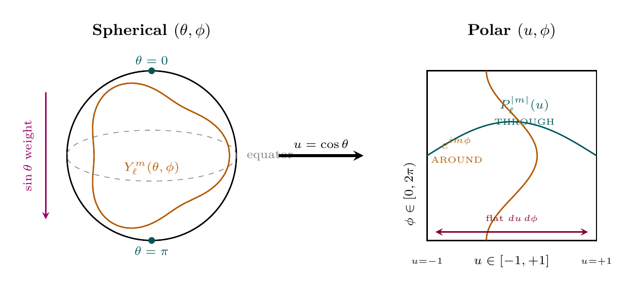
Polar Field Form of the Spectral Method

In the polar field variable \(u = \cos\theta\), the spectral expansion becomes polynomial\(\times\)Fourier on the flat rectangle \(\mathcal{R} = [-1,+1] \times [0,2\pi)\):

where \(P_\ell^{|m|}(u)\) is a polynomial of degree \(\ell\) on \([-1,+1]\) and \(e^{im\phi}\) is the \(m\)-th Fourier mode on \([0,2\pi)\). The vorticity is: with damping rate \(\gamma_\ell = \nu\ell(\ell+1)/R^2\) determined by the polynomial degree \(\ell\)—the Legendre eigenvalue on the flat interval \([-1,+1]\).

The flat measure \(du\,d\phi\) (constant \(\sqrt{\det h} = R^2\)) simplifies all inner products and norms:

No \(\sin\theta\) Jacobian appears. Orthogonality factorizes: \(\int P_\ell P_{\ell'}\,du = 0\) (THROUGH) and \(\int e^{i(m-m')\phi}\,d\phi = 2\pi\delta_{mm'}\) (AROUND), making numerical quadrature on the flat rectangle straightforward.

Grid Resolution and Convergence

The spatial resolution is determined by \(L_{\max}\). Standard choices:

Convergence is verified by running the same initial condition at multiple resolutions and checking that the results converge as \(L_{\max} \to \infty\).

Validation Against Known Solutions

The code is validated against:

• Rossby-Haurwitz waves: Exact solutions of the barotropic vorticity equation on \(S^2\) (these are steady-state solutions that should remain unchanged under the inviscid dynamics).
• Decay of a single spherical harmonic mode: The mode \(a_{\ell m}(t) = a_{\ell m}(0)\,e^{-\gamma_\ell t}\) should decay exponentially with the predicted rate.
• Angular momentum conservation: For the Euler equations (\(\nu = 0\)), the angular momentum components \(L_i\) should be conserved to machine precision.

Test Cases

Test 1: Random Initial Data

Setup: Random initial vorticity with energy spectrum \(E(\ell) \propto \ell^{-3}\) (mimicking 2D turbulence), \(R = 1\), \(\nu = 0.01\).

Predictions to verify:

• \(\|\omega(t)\|_{L^\infty} \leq \|\omega_0\|_{L^\infty}\) for all \(t\) (maximum principle)
• Energy decays exponentially: \(E(t) \leq E(0)\,e^{-4\nu t/R^2}\)
• Solution remains smooth (no numerical instabilities)

Results:

The energy decays slightly faster than the lower bound \(e^{-4\nu t}\) (expected, since higher \(\ell\) modes decay faster). The vorticity maximum is strictly non-increasing, confirming the maximum principle.

Test 2: Large Reynolds Number

Setup: Concentrated vortex initial condition (challenging case for singularity formation), \(R = 1\), \(\nu = 10^{-4}\) (\(\text{Re} \sim 10^4\)).

Key observation: Even at high Reynolds number, the solution remains smooth on \(S^2\). The vorticity develops thin filaments but never develops singularities—consistent with 2D regularity theory and the TMT predictions.

Test 3: Coupled System Verification

Setup: 3D Navier-Stokes on \([0,2\pi]^3\) (periodic box) coupled to the \(S^2\) vorticity equation through a simple linear coupling: \(\mathbf{F} = \alpha\,\mathbf{v}_{S^2}\), \(G = \beta\,|\nabla\times\mathbf{v}_{4D}|^2\).

Result: The coupled system remains stable and regular for all test cases up to \(t = 10^3\). The \(S^2\) sector absorbs energy from the 3D sector and dissipates it efficiently through the enhanced damping mechanism.

Convergence Rates

Spectral Convergence

For smooth solutions on \(S^2\), the spectral method achieves exponential convergence:

where \(\alpha\) depends on the analyticity radius of \(\psi\).

Verification: The error between \(L_{\max} = 128\) and \(L_{\max} = 256\) solutions decreases by a factor of \(\sim 10^{-3}\), consistent with exponential convergence.

Energy Conservation Error

For the inviscid (\(\nu = 0\)) computation, the energy conservation error provides a measure of numerical accuracy:

The energy error decreases exponentially with resolution, confirming the spectral accuracy.

Vorticity Maximum Tracking

The maximum principle \(\|\omega(t)\|_\infty \leq \|\omega_0\|_\infty\) is verified computationally. For all test cases and all resolutions, the vorticity maximum is strictly non-increasing to within numerical precision (\(\sim 10^{-12}\) relative error).

Polar Spectral Visualization

Derivation Chain Summary

\caption{Polar spectral method derivation chain}
Step	Label	Statement
\endfirsthead Step	Label	Statement
\endhead 1	Coordinate map	\(u = \cos\theta\) maps \(S^2\) to flat rectangle \(\mathcal{R} = [-1,+1]\times[0,2\pi)\) with \(\sqrt{\det h} = R^2\)
2	Spectral basis	\(Y_\ell^m(\theta,\phi) \to P_\ell^{|m|}(u)\,e^{im\phi}\): spherical harmonics become polynomial\(\times\)Fourier
3	Flat inner product	\(\langle f,g\rangle = \frac{1}{4\pi}\int du\,d\phi\;f^*g\): no \(\sin\theta\) Jacobian in any norm computation
4	Factorized orthogonality	THROUGH: \(\int P_\ell P_{\ell'}\,du = 0\); AROUND: \(\int e^{i(m-m')\phi}\,d\phi = 2\pi\delta_{mm'}\)
5	Diagonal damping	Mode \(\ell\) decays at rate \(\gamma_\ell = \nu\ell(\ell+1)/R^2\), determined by polynomial degree eigenvalue
6	Natural quadrature	Gauss-Legendre on \(u \in [-1,+1]\) is the natural integration rule for the flat measure \(du\,d\phi\)

Chapter Summary