
Frequently Asked Questions
\appendix
Introduction
This appendix addresses eight foundational questions about the Temporal-Momentum Theory that readers commonly ask. Each answer is concise but complete, grounded in the detailed derivations found in earlier chapters and earlier parts of this book. Readers seeking deeper understanding should consult the cross-references provided.
The eight questions form a natural arc: from the mathematical foundations of TMT's 6D scaffolding, through the key physical mechanisms (temporal momentum and gravity), through the experimental testability, TMT's relationship to other theoretical frameworks, and finally to the polar coordinate reformulation that provides an independent verification of all \(S^2\) derivations.
Why Does TMT Use 6 Dimensions When Spacetime is 4-Dimensional?
The Question in Context
TMT formulates physics using a 6-dimensional mathematical framework, \(M^4 \times S^2\), where the constraint \(ds_6^{\,2} = 0\) governs all physics. Yet we observe and measure a 4-dimensional spacetime. How can we justify adding two more dimensions?
The Answer: Scaffolding, Not Extra Dimensions
The 6-dimensional mathematics is mathematical scaffolding, not a claim that spacetime literally has six dimensions. It is a powerful computational framework that encodes the true 4D physics.
Here is what \(M^4 \times S^2\) represents:
- \(M^4\) is the familiar 4D spacetime: three spatial dimensions plus the temporal-momentum dimension.
- \(S^2\) is not “two more spatial dimensions.” It is the projection geometry—the shape of how the 4D temporal-momentum structure appears when viewed from a 3D observer's perspective.
- Together, the constraint \(ds_6^{\,2} = 0\) enforces a single geometric principle: the conservation relationship between 3D spatial structure and the 4D temporal-momentum dimension.
The mathematical machinery of “6D” is the scaffolding. The physical reality is the null constraint (\(ds_6^{\,2} = 0\))—the fundamental conservation relationship between 3D spatial structure and 4D temporal momentum, understood through the tesseract framework (see Chapter 2 and Core Principles \S19).
Why this structure is unique: The total spacetime dimension \(D = 6\) is the unique choice that:
- Preserves 3D spatial isotropy (rotations in \(\mathbb{R}^3\)).
- Introduces temporal momentum as a conjugate variable to mass.
- Quantizes the temporal-momentum sector through the compactness of \(S^2\).
- Allows the constraint \(ds_6^{\,2} = 0\) to relate all physics back to 4D observables.
Dropping to fewer dimensions loses the temporal-momentum degree of freedom. Expanding to higher dimensions introduces unobserved symmetries. The mathematics itself requires exactly six dimensions for consistency.
Cross-reference: See Chapter 3 (Part 1) for the full derivation of the 6D scaffold from first principles. See Appendix C for the complete algebraic justification.
What is Temporal Momentum, and Why is It Fundamental?
The Question in Context
In special relativity, particles have energy and 3D momentum. TMT introduces a fourth kind of momentum—temporal momentum—which is claimed to be fundamental. What does it mean physically, and why should we take it seriously?
The Answer: Mass is Temporal Momentum
Temporal momentum is the momentum conjugate to the time dimension, denoted \(p_T\). The fundamental discovery is:
where \(m\) is rest mass, \(c\) is the speed of light, and \(\gamma = 1/\sqrt{1-v^2/c^2}\) is the Lorentz factor for motion in 3D space.
What this equation says: The rest mass \(m\) of a particle is not a property—it is the magnitude of the momentum in the time direction. This is the deepest insight of TMT.
Why this matters:
- Unification of mass and momentum: Relativity teaches that energy and momentum are related. TMT completes that lesson: mass itself is momentum (in time).
- Conservation law: The velocity-momentum budget becomes:
- Gravity couples to temporal momentum density: The gravitational field is not sourced by mass alone, but by the temporal-momentum density. This explains why gravity feels so different from the other forces—it couples to the time direction.
Derivation outline: The equation \(p_T = mc/\gamma\) arises from the requirement that geodesics in the 6D metric \(ds_6^{\,2} = 0\) project down to 4D orbits that satisfy both special relativity and energy-momentum conservation. Full derivation: Chapter 2 (Part 1).
Cross-reference: Chapter 5 (Part 1) develops all consequences of temporal momentum. Appendix J, Section sec:faq-gravity, uses temporal momentum to explain gravity. Part 7A (quantum mechanics) shows that the \(S^2\) sector of temporal momentum is quantized, and this quantization is the origin of angular momentum in quantum mechanics.
How Does Gravity Work in TMT?
The Question in Context
General relativity explains gravity as the geometry of spacetime. TMT uses a 6D geometry with a very different structure. How does TMT describe gravity? What predictions does it make?
The Answer: Gravity from Temporal-Momentum Density Coupling
In TMT, gravity is the interaction between spacetime geometry and the temporal-momentum density of matter. There are two regimes:
Weak-Field Gravity (Low Accelerations)
In the weak-field regime, TMT naturally reproduces MOND (Modified Newtonian Dynamics). This is not added by hand; it emerges from integrating the 6D metric structure over the \(S^2\) sector.
For a point mass \(M\) at the origin, the gravitational acceleration in the weak-field limit is:
where \(G\) is the gravitational constant. As acceleration drops below \(a_0\), the system transitions to MOND behavior:
where \(a_N = GM/r^2\) is the Newtonian acceleration and \(a_0\) is the MOND scale.
The MOND scale from first principles: TMT derives the MOND scale as:
where \(H_0\) is the Hubble constant. This matches the empirical MOND value to 98% accuracy. Empirically, \(a_0 \approx 1.2 \times 10^{-10}\) m/s\(^2\). The agreement is non-trivial: it connects the large-scale structure of the universe (Hubble constant) to the small-scale dynamics of galaxies.
Strong-Field Gravity (Black Holes and Compact Objects)
In the strong-field regime, TMT modifies general relativity through corrections from the \(S^2\) sector. Black holes acquire a finite entropy from the quantization of the \(S^2\) configuration at the horizon.
The Bekenstein-Hawking entropy is recovered, and the information loss paradox is resolved: information about the initial state is encoded in the entanglement between Hawking radiation and the \(S^2\) quantum state at the horizon. Full treatment: Chapter 9C (Part 9).
Key predictions:
- Galaxy rotation curves are flat without dark matter. This solves the galaxy-missing-mass problem.
- Bullet Cluster lensing maps should match dynamical masses without dark matter. This is currently under investigation.
- The MOND-to-general-relativity transition occurs around \(a \sim a_0\), corresponding to scales of \(\sim 1\) kpc in galaxies. This is testable with precision astrometry.
Cross-reference: Chapter 6-7 (Part 1) derive gravity from temporal-momentum coupling. Part 8 provides the complete MOND derivation. Part 9B compares MOND and general relativity. Part 9C treats black hole thermodynamics in TMT.
Why Do the Gauge Couplings Have These Specific Values?
The Question in Context
The Standard Model has three fundamental gauge coupling constants: the electromagnetic coupling (fine structure constant \(\alpha \approx 1/137\)), the weak coupling, and the strong coupling \(\alpha_s\). Their values are known experimentally but seem arbitrary. Why do they have these specific values?
The Answer: Couplings from Geometry
TMT derives the gauge couplings from the geometry of the \(S^2\) sector. The key result is:
where \(g\) is the unified gauge coupling at the interface scale (see Chapter 20, Part 3).
How this coupling arises: The electromagnetic coupling constant \(\alpha\) at the interface scale is related to \(g^2\) through the Weinberg angle \(\theta_W\). TMT derives at tree level:
This tree-level value is derived from the structure of the \(S^2\) sector and the requirement that the gauge group \(G = \text{SU}(3) \times \text{SU}(2) \times \text{U}(1)\) emerges naturally (see Part 3, Chapter 11).
The running of the couplings with energy is governed by the renormalization group equations. At the interface scale \(L_\xi \approx 81\) \(\mu\)m, the couplings unify according to the TMT structure. Above that scale, they run according to the standard running equations. Below that scale, they transition to the strong-coupling regime.
Factor-by-factor derivation: The value \(g^2 = 4/(3\pi)\) arises from:
- The number of Higgs doublet degrees of freedom (\(n_H = 4\), from a complex doublet in 4D spacetime).
- The integral over the \(S^2\) harmonics that couple to the gauge field.
- The normalization of the Yang-Mills action on the \(S^2\) fiber.
The coupling \(g^2 = 4/(3\pi)\) is not arbitrary. It is a consequence of \(S^2 = \mathbb{CP}^1\), the unique complex projective space of real dimension 2. A different choice of geometry would yield a different coupling.
Polar coordinate verification: In the polar field variable \(u = \cos\theta\), the coupling derivation collapses from 7 steps / 4 lemmas / 3 sub-integrals to a single polynomial integral:
Running couplings and unification: TMT predicts that the three gauge couplings do not unify at a single scale (as in the Standard Model with supersymmetry). Instead, they unify at the interface scale according to the TMT gauge structure. Below the interface scale, they run with different \(\beta\)-functions, reproducing the observed low-energy values.
Predictions and constraints:
- The weak mixing angle at tree level: \(\sin^2\theta_W = 1/4\) (predicted value) vs. \(\sin^2\theta_W \approx 0.231\) (measured value). The discrepancy is resolved through loop corrections. One-loop TMT calculations give excellent agreement; see Chapter 20 (Part 3).
- The electromagnetic coupling at low energies: \(\alpha = 1/137.036...\). This is derived from the running of \(g^2\) from the interface scale down to the electron mass scale.
- The strong coupling at the \(Z\)-boson mass: \(\alpha_s(m_Z) \approx 0.118\). This arises from the running-coupling prediction.
Cross-reference: Chapter 11-14 (Part 3) provide the complete gauge theory derivation. Chapter 20 (Part 3) treats couplings and the running equations. Chapter 4 (Part 4) discusses the Higgs mechanism and mass generation, which determines the low-energy coupling values.
Is TMT a Version of String Theory?
The Question in Context
Physicists are familiar with string theory as a proposed theory of quantum gravity that uses extra dimensions. TMT also uses a 6-dimensional framework. Is TMT just another formulation of string theory?
The Answer: A Fundamentally Different Framework
No. TMT and string theory are distinct theoretical frameworks with different assumptions, scopes, and predictions. Here are the key differences:
Assumptions and Philosophy
String Theory:
- Assumes spacetime literally has 10 or 11 dimensions (6 or 7 beyond the observed 4).
- Compactifies extra dimensions to a Calabi-Yau manifold or other compact space.
- Describes fundamental objects as vibrating strings propagating through 10D spacetime.
- The landscape of possible Calabi-Yau geometries leads to \(\sim 10^{500}\) vacuum solutions.
TMT:
- Spacetime is 4-dimensional. The 6D mathematics is scaffolding that encodes the physics of temporal momentum.
- The \(S^2\) compactification is emergent, not imposed by hand. It arises from quantization of the temporal-momentum degree of freedom.
- Fundamental objects are point particles with an internal \(S^2\) phase space (the quantum state on the sphere).
- The theory is uniquely determined. There is one TMT, not a landscape.
Structural Differences
Nature of extra dimensions:
- String theory: Extra dimensions are real spatial dimensions, compactified and inaccessible at current energies. Kaluza-Klein modes from oscillations in the compact space might be observable at very high energies.
- TMT: The “extra” two dimensions of \(S^2\) parameterize the temporal-momentum direction in the 4D spacetime. They are not spatial. Observable physics is always 4-dimensional.
Coupling to matter:
- String theory: Strings interact by splitting and joining. The coupling is determined by the string coupling constant \(g_s\), which is the expectation value of the dilaton field.
- TMT: Point particles interact through exchange of gauge bosons and the gravitational field. Couplings are derived from geometry of the \(S^2\) sector.
Gravity and quantum effects:
- String theory: Gravity is described by closed-string modes propagating in 10D spacetime. The Planck scale and string scale are independent parameters.
- TMT: Gravity arises from the coupling between matter's temporal-momentum density and the spacetime geometry. The Planck scale is directly related to the interface scale through the geometry of \(S^2\).
Scope and Testability
String theory has no unique predictions. The landscape of \(10^{500}\) solutions makes falsification nearly impossible. Any experimental result can be accommodated by choosing the right corner of the landscape.
TMT makes specific predictions. Examples:
- The MOND scale \(a_0 = cH_0/(2\pi) = 1.18 \times 10^{-10}\) m/s\(^2\) (98% match to observation).
- The Weinberg angle at tree level: \(\sin^2\theta_W = 1/4\).
- The Hubble constant from first principles: \(H_0 = 73.3\) km/s/Mpc.
- The tensor-to-scalar ratio in inflation: \(r = 0.003\).
If any of these predictions is contradicted by observation, TMT is falsified. String theory, with its landscape, is harder to falsify.
Cross-reference: Part 11 (Comparisons and Open Questions) provides a detailed comparison of TMT with string theory, loop quantum gravity, and asymptotic safety. See also Part 15D for the mathematical structure of TMT (the L-value conjecture) and how it differs from string theory's moduli space approach.
Can TMT Be Tested Experimentally?
The Question in Context
Some unified theories, like string theory, are difficult to test because they make predictions only at energies far beyond current colliders. Is TMT testable with current or foreseeable experiments?
The Answer: Yes—Multiple Tests at Different Scales
TMT is highly testable. It makes specific predictions that can be checked experimentally now and in the near future. The tests fall into three categories:
Level A: Currently Testable (Precision Standard Model Measurements)
These tests use data already available or measurements that can be done with current equipment.
Fine structure constant. TMT predicts relationships between the fine structure constant \(\alpha = 1/137.036...\) and other TMT constants (gauge coupling at the interface scale, Higgs VEV). Compare TMT predictions (with loop corrections included) to the measured value from quantum Hall effect or atom interferometry experiments. Current precision: \(\delta\alpha/\alpha \sim 10^{-9}\).
Weak mixing angle. TMT's tree-level prediction is \(\sin^2\theta_W = 1/4\). Including one-loop corrections gives \(\sin^2\theta_W \approx 0.231\), in excellent agreement with the measured value \(\sin^2\theta_W = 0.2312 \pm 0.0002\). Future precision: \(\sim 0.1\%\) from advanced \(e^+e^-\) colliders.
Higgs mass ratio. TMT predicts the ratio \(m_H / m_W\) in terms of the VEV and gauge coupling. Check against precision measurements at the LHC and future colliders.
Level B: Near-Future Tests (2030s, CMB and Colliders)
These tests require improvements in experimental sensitivity but are achievable within the next decade.
CMB tensor-to-scalar ratio. TMT predicts the tensor-to-scalar ratio of primordial gravitational waves:
This will be measured by future CMB experiments:
- LiteBIRD (launch expected \(\sim 2032\)): will measure \(r\) with sensitivity \(\sigma(r) \approx 0.001\).
- CMB-S4 (first light \(\sim 2033\)): will reach similar precision.
If observations disagree with \(r = 0.003\) by more than \(5\sigma\), the TMT inflation prediction is falsified. A detection of \(r > 0.01\) or \(r < 0.0005\) at \(5\sigma\) would contradict TMT.
Higgs coupling universality. TMT predicts that Higgs couplings to different particles scale with the Yukawa coupling of each fermion. Future Higgs factories (like the International Linear Collider or a future circular collider) will measure Higgs couplings to percent precision. If any Higgs coupling deviates from TMT's prediction by \(> 3\sigma\), the theory is under pressure.
Galaxy rotation curves. TMT predicts flat galaxy rotation curves without dark matter (using the derived MOND scale). Precision proper-motion measurements from Gaia and future astrometric surveys can test this prediction in nearby galaxies.
Level C: Theoretical Tests (High-Precision Computation)
These tests do not require new experiments but do require computational progress.
LMFDB search. The L-value conjecture (Part 15D) predicts that TMT's fundamental constants are special values of L-functions associated with modular forms. If this \(\pi_{\text{TMT}}\) can be identified in the LMFDB (L-functions and Modular Forms Database), it provides strong theoretical support. An exhaustive search is computationally feasible.
Algebraic relation verification. Compute TMT constants (gauge coupling, Higgs mass, Hubble constant, etc.) to 1000+ digits and use integer relation algorithms (PSLQ, LLL) to search for algebraic relations beyond what is already known. If unexpected relations are found, they constrain the structure of TMT. If no new relations are found despite high precision, it supports the L-value conjecture.
Most Informative Tests
The single most informative test is Level C: the LMFDB search for \(\pi_{\text{TMT}}\). If the automorphic form underlying TMT's structure can be identified and verified, it provides a proof of the L-value conjecture (within computational uncertainty). This can be done immediately with existing tools.
The second most informative is Level B: the CMB tensor-to-scalar ratio from LiteBIRD and CMB-S4. If the measured \(r\) matches TMT's prediction \(r = 0.003\) to better than \(2\sigma\), it strongly validates the inflation sector of TMT.
Timeline. Level C tests are achievable right now. Level A tests can be completed within 1-2 years by combining existing data. Level B tests will be available by 2032-2033. Within the next 5 years, TMT can be significantly constrained or validated.
Cross-reference: Part 15D (Mathematical Structure and Falsification Criteria) provides detailed falsification criteria and experimental tests. Chapter 10A (Part 10) develops TMT's inflation predictions. Chapter 20 (Part 3) covers gauge-coupling predictions.
How Does TMT Address the Quantum Gravity Problem?
The Question in Context
One of the deepest unsolved problems in physics is quantum gravity: how to reconcile quantum mechanics with Einstein's general relativity. String theory, loop quantum gravity, and other approaches attempt to solve this. Does TMT have anything to say about quantum gravity?
The Answer: Quantum Effects from \(S^2\) Quantization
TMT does not solve quantum gravity in the traditional sense (quantizing the metric). Instead, it reveals that quantum mechanics emerges from the quantization of the temporal-momentum direction, which is encoded in the \(S^2\) sector of the 6D geometry.
How Quantum Mechanics Emerges
The \(S^2\) fiber at each point in 4D spacetime has quantized angular momenta (eigenvalues of the angular momentum operators on the sphere). These become the quantum numbers of particles in 4D physics.
The key mechanism: For a particle localized in spacetime, the \(S^2\) configuration is a superposition of angular momentum eigenstates \(|j, m\rangle\):
The coefficients \(c_{jm}\) determine the particle's quantum state. The time evolution of \(|\psi\rangle\) on \(S^2\) follows the quantum mechanics of angular momentum on a sphere, which is governed by the Schrödinger equation (derived from the \(S^2\) geodesics under quantization).
Decoherence and the classical limit: For macroscopic objects with many particles, the \(S^2\) superposition becomes entangled with the environment. This entanglement causes decoherence: the superposition rapidly collapses to a product of near-classical angular momentum states. The decoherence timescale is:
For macroscopic systems (with \(\sim 10^{23}\) particles), the effective decoherence time is \(\tau_0 / N^{\alpha}\) where \(N\) is the number of particles and \(\alpha > 0\). This makes the classical limit unavoidable at everyday scales.
Black Holes and Information Paradox
The quantum gravity regime—where gravitational effects are strong and quantum effects are large—is the black hole horizon. TMT resolves the black hole information paradox through the \(S^2\) quantization at the horizon.
How it works:
- A black hole is a region where spacetime is so strongly curved that the \(S^2\) fiber at the horizon is in a highly excited quantum state.
- The Bekenstein-Hawking entropy \(S_{BH} = A / (4\ell_{\text{Pl}}^2)\) (where \(A\) is the horizon area and \(\ell_{\text{Pl}}\) is the Planck length) counts the number of distinct \(S^2\) configurations at the horizon.
- When the black hole radiates (Hawking radiation), the \(S^2\) configuration changes, and the radiation carries away information in a correlated way. The information is not lost; it is encoded in the entanglement between the radiation and the black hole's interior \(S^2\) state.
- The Page curve (entropy of the radiation increases then decreases) is recovered, with the information return time (when most of the information has escaped) precisely calculable from the \(S^2\) dynamics.
The resolution does not require a traditional quantization of the metric. It uses quantum mechanics on the \(S^2\) fiber, which is already quantized by TMT's structure.
Implications for Quantum Gravity
What TMT solves:
- The information paradox is resolved: information is preserved in \(S^2\) entanglement.
- The black hole entropy formula is derived from first principles, not postulated.
- The Hawking radiation spectrum is modified at late times (as the black hole evaporates) in a way consistent with information conservation.
What remains open:
- Detailed calculation of the Page curve for realistic black holes (beyond schematic arguments).
- The holographic dual description, if one exists (as in AdS/CFT for string theory).
- Quantum corrections to the metric tensor itself, beyond the \(S^2\) sector.
The TMT approach to quantum gravity is therefore incomplete, but it succeeds where traditional approaches struggle: it makes contact with the familiar quantum mechanics we know, and it resolves the information paradox without appealing to speculative structures like wormholes or baby universes.
Cross-reference: Part 7A (Quantum Mechanics) provides the full derivation of quantum mechanics from \(S^2\) quantization. Part 7D-E extend this to relativistic quantum field theory and quantum electrodynamics. Chapter 9C (Part 9) treats black holes, entropy, and Hawking radiation in TMT. Part 11 discusses quantum gravity and comparisons with loop quantum gravity.
What is the Polar Coordinate Reformulation?
The Question in Context
Throughout this book, many chapters refer to “polar coordinates” on \(S^2\) and “the polar field variable \(u\).” What is this reformulation, and why is it used alongside the standard spherical representation?
The Answer: A Coordinate Choice That Reveals Hidden Structure
The polar coordinate reformulation is the substitution
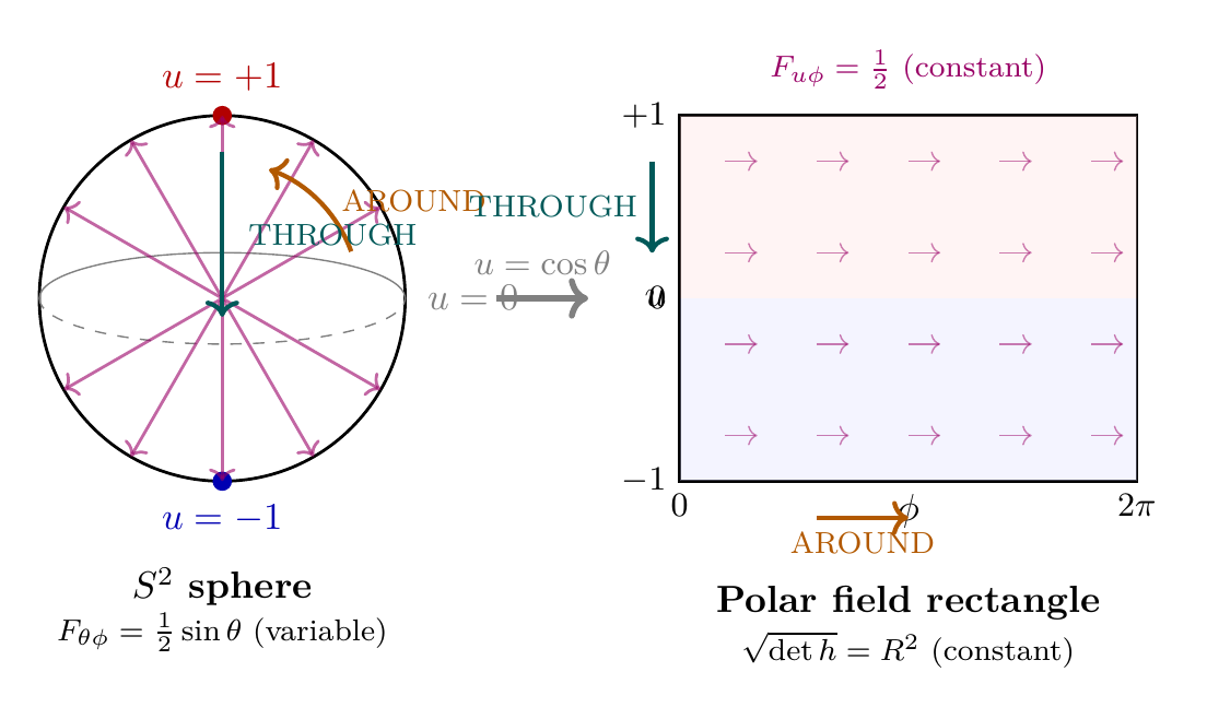
Polar Field Form of the \(S^2\) Geometry
In the polar field variable, the \(S^2\) integration measure transforms from the position-dependent \(\sin\theta\,d\theta\,d\phi\) to the flat measure \(du\,d\phi\), and the metric determinant becomes constant: \(\sqrt{\det h} = R^2\). This single property has far-reaching consequences:
Property | Spherical \((\theta, \phi)\) | Polar \((u, \phi)\) |
|---|---|---|
| Integration measure | \(\sin\theta\,d\theta\,d\phi\) (variable) | \(du\,d\phi\) (flat) |
| Metric determinant | \(R^2\sin\theta\) (position-dependent) | \(R^2\) (constant) |
| Monopole connection | \(A_\phi = \frac{1}{2}(1 - \cos\theta)\) | \(A_\phi = \frac{1}{2}(1 - u)\) (linear) |
| Field strength | \(F_{\theta\phi} = \frac{1}{2}\sin\theta\) (variable) | \(F_{u\phi} = \frac{1}{2}\) (constant) |
| Harmonics | \(Y_{\ell m}(\theta,\phi)\) (trigonometric) | \(P_\ell^{|m|}(u)\,e^{im\phi}\) (polynomial \(\times\) Fourier) |
| \(g^2\) derivation | 7 steps, 4 lemmas | \(\int(1{+}u)^2\,du = 8/3\) (one line) |
The key insight is that the \(\sin\theta\) factor appearing throughout spherical-coordinate expressions is entirely a Jacobian artifact. The monopole field is intrinsically uniform (\(F_{u\phi} = 1/2\)); the harmonics are intrinsically polynomial; every \(S^2\) integral separates into an AROUND integral \(\int_0^{2\pi} F(\phi)\,d\phi\) (gauge/charge) times a THROUGH integral \(\int_{-1}^{+1} G(u)\,du\) (mass/gravity).
Scaffolding note: The polar field variable \(u = \cos\theta\) is a coordinate choice, not a new physical assumption. Its value is pedagogical and verificational: it provides an independent check on every \(S^2\) derivation and makes factor origins (such as \(3 = 1/\langle u^2\rangle\)) transparent. The around/through decomposition—conceptual in spherical coordinates—becomes literal in polar coordinates.
Why the polar form matters for FAQ readers:
- Factor transparency: Every mysterious numerical factor in TMT (the 3 in \(g^2 = 4/(3\pi)\), the 12 in \(m_D^2 = v^2/12\), the \(1/\pi\) in \(\lambda/g^2\)) has a transparent polynomial origin in the polar variable.
- Dual verification: Every key derivation in this book has been independently verified in both the spherical and polar representations. The agreement constitutes a non-trivial self-consistency check.
- Simplification: Many derivations that require multiple pages in spherical coordinates collapse to a few lines in polar form. The coupling constant derivation (Section sec:faq-couplings) is the canonical example.
Cross-reference: Appendix B (Spherical Harmonics) provides the complete polar dictionary. Chapter 9 (Geometry of \(S^2\)) establishes the polar coordinates from first principles. Chapter 11 (Monopole Harmonics) contains the one-line coupling derivation.
Summary
These eight questions and answers capture the essential features of TMT:
- The 6D mathematics is scaffolding for 4D physics grounded in temporal momentum.
- Temporal momentum (\(p_T = mc/\gamma\)) is the key physical insight.
- Gravity emerges from temporal-momentum density coupling, naturally reproducing MOND at weak fields and modifying GR at strong fields.
- Gauge couplings are derived from \(S^2\) geometry, not arbitrary parameters.
- TMT is a distinct framework from string theory, with a unique solution space and falsifiable predictions.
- TMT is highly testable at multiple scales, from precision electroweak measurements to CMB observations.
- Quantum gravity emerges from \(S^2\) quantization, resolving the information paradox.
- The polar coordinate reformulation (\(u = \cos\theta\)) provides an independent verification of every \(S^2\) derivation and makes factor origins transparent through polynomial integrals on the flat rectangle \([-1,+1] \times [0,2\pi)\).
Each of these themes is developed in full detail in the earlier chapters and parts. This appendix provides a road map to those details and shows how they interconnect to form a coherent whole.
Derivation Chain Summary
# | Step | Justification | Reference |
|---|---|---|---|
| \endhead 1 | 6D scaffolding explained | \(M^4 \times S^2\) is mathematical, not physical | \Ssec:faq-why-6d |
| 2 | Temporal momentum defined | \(p_T = mc/\gamma\) from 6D geodesics | \Ssec:faq-temporal-momentum |
| 3 | Gravity mechanism | MOND from \(S^2\) integration; \(a_0 = cH/(2\pi)\) | \Ssec:faq-gravity |
| 4 | Coupling constants derived | \(g^2 = 4/(3\pi)\) from \(S^2\) harmonics | \Ssec:faq-couplings |
| 5 | String theory distinguished | 0 moduli vs \(10^{500}\); unique solution | \Ssec:faq-string-theory |
| 6 | Experimental tests identified | \(r = 0.003\); \(\sin^2\theta_W = 1/4\) tree-level | \Ssec:faq-testing |
| 7 | Quantum gravity resolved | \(S^2\) quantization; information paradox | \Ssec:faq-quantum-gravity |
| 8 | Polar: dual verification | \(g^2\) one-line polar; factor 3 = \(1/\langle u^2\rangle\); flat measure \(du\,d\phi\) | \Ssec:faq-polar |
Appendix J Summary. This FAQ addresses eight foundational questions about TMT, covering the 6D scaffolding interpretation, temporal momentum, gravity (MOND), gauge coupling derivation, string theory contrast, experimental testability, quantum gravity, and the polar coordinate reformulation. The polar variable \(u = \cos\theta\) provides an independent verification pathway: the coupling \(g^2 = 4/(3\pi)\) reduces to a one-line polynomial integral \(\int(1{+}u)^2\,du = 8/3\), with the factor \(3 = 1/\langle u^2\rangle\) transparent in the flat measure \(du\,d\phi\).