
Kaluza-Klein Theory
Opening Remarks
This appendix develops Kaluza-Klein (KK) theory as the classical framework against which the Temporal Momentum Theory (TMT) is compared. The presentation is complete and self-contained: all derivations are shown step by step, every numerical factor traced to its source, and the physical interpretation given at each stage. The critical insight is this: TMT is not Kaluza-Klein theory. The mathematical scaffolding of \(S^{2}\) in TMT serves to derive 4D physics, not to describe literal extra spatial dimensions. Understanding classical KK first makes this distinction clear.
Roadmap: This appendix establishes the classical KK framework (§app:kk-classical), derives the KK matching condition from the interface principle (§app:kk-matching), computes the tower spectrum explicitly (§app:kk-tower), applies phenomenological constraints (§app:kk-pheno), and finally explains why TMT succeeds where classical KK fails (§app:kk-vs-tmt).
—
Classical Kaluza-Klein Theory
Historical Setup and Core Idea
The classical Kaluza-Klein theory, developed in the 1920s (Kaluza 1921, Klein 1926), proposes that electromagnetism can be understood as gravity in a five-dimensional spacetime. The fifth dimension is “compactified” — confined to a circle of radius \(R\) — and this compactification gives rise to the electromagnetic gauge field when observed in the effective 4D theory.
The Core Construction:
Begin with a 5D metric:
where:
- \(\mu, \nu \in \{0, 1, 2, 3\}\) label 4D spacetime coordinates
- \(\xi \in [0, 2\pi)\) is the fifth (compact) coordinate
- \(g_{\mu\nu}(x)\) is the 4D metric (identified with the graviton)
- \(A_{\mu}(x)\) is a 4D vector field (identified with the electromagnetic potential)
- \(\phi(x)\) is a scalar field (the dilaton, related to the radion)
This metric is called block diagonal because it separates the 4D geometry from the compact direction. The key insight is that the \(A_{\mu}\) term mixing \(x\) and \(\xi\) directions creates a “twist” — this is where gauge structure emerges geometrically.
The 5D Einstein Action
The action in 5D is the Einstein-Hilbert action:
where \(M_{5}\) is the 5D Planck mass, \(g_{5}\) is the determinant of the 5D metric, and \(R_{5}\) is the 5D Ricci scalar. The matter Lagrangian \(\mathcal{L}_{\text{matter}}\) is defined on the 5D manifold.
The Integration Step:
To get the 4D effective action, integrate over the compact coordinate \(\xi\):
The integral \(\int_{0}^{2\pi} d\xi\) over the compact dimension produces a volume factor \(V_{\text{compact}} = 2\pi R\). This is the origin of the KK coupling formula.
Derivation of the 4D Coupling
Step 1: Dimensional Reduction
The 5D Ricci scalar \(R_{5}\) can be decomposed into 4D and cross terms. The detailed computation (involving Christoffel symbols for the metric eq:5d-metric-kk) yields:
where \(F_{\mu\nu} = \partial_{\mu}A_{\nu} - \partial_{\nu}A_{\mu}\) is the electromagnetic field strength, and \(g_{4} = \det(g_{\mu\nu})\).
Step 2: Volume Integral
Integrating over \(\xi\) from 0 to \(2\pi\) (with constant \(R\) and assuming \(\phi, A_{\mu}\) are independent of \(\xi\)):
Step 3: Rescaling and the Coupling Formula
The 4D action becomes:
Define the 4D Planck mass by absorbing the compact volume:
and the 4D gauge coupling from the kinetic term. Rewriting the electromagnetic term in standard form \(-\frac{1}{4g^{2}} F^{2}\) yields:
where \(\phi^{2}_{\text{ave}}\) represents the average dilaton value.
For the simplest KK model with constant dilaton (\(\phi = \text{const}\)), this becomes:
This is the fundamental KK formula: the 4D gauge coupling is suppressed by the volume of the compact space.
Numerical Application of Classical KK
To test whether classical KK predicts the observed gauge coupling, substitute the measured scales.
Input Parameters:
From TMT Part 2, we identify \(R = L_{\xi}/(2\pi)\) where \(L_{\xi} \approx 81 \, \mu\text{m}\) is the interface scale:
In natural units (\(\hbar = c = 1\)), this becomes:
Using \(\hbar c = 197.3 \, \text{MeV} \cdot \text{fm} = 197.3 \times 10^{-15} \, \text{MeV} \cdot \text{m}\):
Coupling Calculation:
Assuming \(g_{5} \sim O(1)\) (a natural choice in the 5D theory):
Computing numerically:
But this must be dimensionless in the 4D effective theory. The proper formula accounts for the ratio of scales:
With \(\ell_{\text{Pl}} \approx 1.6 \times 10^{-35} \text{ m}\) and \(R \approx 1.3 \times 10^{-5} \text{ m}\):
Therefore:
The Disaster:
The measured weak gauge coupling is \(g^{2} \approx 0.42\). The KK prediction is \(g^{2} \sim 10^{-60}\). This is a discrepancy of approximately 60 orders of magnitude. Classical Kaluza-Klein theory fails catastrophically.
—
KK Matching and the Interface Principle
Why KK Fails: The Physical Reason
The failure of classical KK is not accidental or due to missing factors. It is a consequence of the fundamental assumptions in the KK approach.
The KK Picture:
In classical KK, the coupling is computed by:
- Writing a 5D action with fields “propagating freely” through the compact dimension
- Integrating the action over the compact space to get an effective 4D action
- The volume of the compact space appears in the denominator, suppressing the coupling
This works for fields that genuinely propagate through a 3D bulk space. For example, if you have a wave in a fiber optic cable, the power per unit cross-section (coupling strength) decreases as the fiber gets thicker.
The Problem:
But the Higgs field is not propagating freely through the compact dimension. Instead, as shown in Part 2 of TMT, the Higgs field is a section of a non-trivial U(1) bundle. The monopole topology forces the field to be localized on the interface \(S^2\), not spread throughout a 3D volume.
The Theorem:
For a gauge-Higgs system on \(S^2\) with a monopole (non-trivial U(1) bundle of first Chern class):
- The Higgs field is a section of the line bundle \(L^{1/2} \to S^2\), not a function
- Sections cannot extend smoothly through any 3D bulk filling (Dirac string singularity)
- The coupling is determined by section overlaps on \(S^2\), not bulk integrals
- The KK formula \(g^{2} \sim 1/\text{Vol}\) does not apply
Case 1: Trivial Bundle (No Monopole)
If the bundle is trivial, the Higgs field \(H\) is an ordinary function:
Any such function can be extended to a continuous map on any 3D ball \(B^{3}\) with boundary \(S^2\):
This is topologically allowed (the first Chern class vanishes for trivial bundles). Integration over the filling volume \(B^{3}\) is well-defined, and the coupling is suppressed by \(\text{Vol}(B^{3}) \sim R^{3}\).
Case 2: Non-Trivial Bundle (Monopole)
If a monopole is present, the first Chern class is \(c_{1} = 1\) (or another nonzero integer). The Higgs field must be a section of \(L^{1/2}\):
The connection \(\mathbf{A}\) (the monopole potential) twists the bundle so that:
where \(\Phi = 2\pi n\) is the total magnetic flux. A single-valued section on \(S^2\) satisfies this.
However, any attempt to extend this section smoothly through a 3D bulk encounters an obstruction. The Dirac string singularity appears at some location — the point where the connection cannot be made single-valued everywhere. To avoid the singularity, the section is confined to \(S^2\) itself.
Mathematically: the extension problem is:
(There is no way to extend the non-trivial line bundle from the boundary to the interior without introducing a singularity.)
Conclusion:
Fields on the monopole-twisted interface cannot propagate through a bulk. They must remain on the 2-dimensional interface \(S^2\). Therefore, the coupling is determined by 2D surface overlaps, not 3D volume integrals. □
The Interface Transmission Coefficient
Since the classical KK volume formula does not apply, a new coupling formula is needed. This is provided by the interface principle.
The Transmission Coefficient:
The interface \(S^2\) acts as a “transmitter” between the 6D mathematical scaffolding and the 4D observable physics. The transmission coefficient is:
This factor of \(3\pi^{2}\) has a precise geometric origin:
| Factor | Value | Origin | Physical Meaning |
|---|---|---|---|
| 3 | \(n_{g}\) | \(\dim(\text{SO}(3))\) | Gauge structure from \(S^2\) isometry |
| \(\pi\) (first) | \(P\) | \(\int_{S^2} |Y_{00}|^{4} d\Omega = 1/\pi\) | Participation ratio (Higgs spreading) |
| \(\pi\) (second) | Loop factor | Quantum corrections, \(n_{\text{H}}\) cancellation | Loop suppression |
The first factor of 3 comes from the gauge group \(\text{SU}(2)\), which emerges from the \(\text{SO}(3)\) isometry of \(S^2\). The second factor of \(\pi\) is the participation ratio, which measures how the Higgs field spreads on the interface. The third factor of \(\pi\) comes from loop integrals.
Polar Field Decomposition of the Transmission Coefficient
In the polar field variable \(u = \cos\theta\), the geometric origin of \(\tau = 1/(3\pi^2)\) becomes transparent. Each factor is a distinct property of the flat rectangle \([-1,+1] \times [0,2\pi)\):
The factor \(3 = 1/\langle u^2\rangle\) is the reciprocal of the second moment of the polar variable:
The factor \(\pi^2\) comes from AROUND-direction geometry: participation ratio \(\pi\) (from the fourth-moment integral \(\int |Y|^4\,du\,d\phi = 1/\pi\)) and loop suppression \(\pi\) (from the \(2\pi\) azimuthal periodicity).
Factor | Value | Polar Origin | Direction |
|---|---|---|---|
| 3 | \(1/\langle u^2\rangle\) | Second moment of \(u\) on \([-1,+1]\) | THROUGH |
| \(\pi\) (first) | \(P = 1/\pi\) | \(\int |Y|^4\,du\,d\phi\) (flat measure) | Mixed |
| \(\pi\) (second) | Loop factor | \(2\pi\) azimuthal periodicity | AROUND |
Scaffolding note: The polar field variable \(u = \cos\theta\) is a coordinate choice, not a new physical assumption. The transmission coefficient \(\tau = 1/(3\pi^2)\) is a geometric property of the \(S^2\) interface, independent of coordinate choice. The polar decomposition makes the THROUGH/AROUND factorization manifest, revealing that the factor of 3 is the reciprocal of a polynomial second moment.
Application:
With this transmission coefficient, the 4D observable physics (VEV and coupling) are determined from the 6D mathematical scaffolding by:
For the specific case of \(v_{\text{6D}} = M_{6} = 7296 \, \text{GeV}\) (derived from modulus stabilization in Part 4):
This matches the observed Higgs VEV to high precision.
The Matching Condition:
The interface principle establishes a one-to-one correspondence between:
- 6D mathematical scaffolding quantities (defined via \(S^{2}\) harmonics and structure)
- 4D observable physics (what is measured in experiments)
This is the KK matching that gives the appendix its name. It is not the classical KK matching (which fails), but a corrected matching that accounts for monopole topology.
—
The Kaluza-Klein Tower Spectrum
Harmonic Decomposition on \(S^{2}\)
Any function on the 2-sphere \(S^2\) can be expanded in spherical harmonics \(Y_\ell m}(\theta, \phi)\), where \(\ell \in \{0, 1, 2, \ldots\) is the angular momentum quantum number and \(m \in \{-\ell, \ldots, +\ell\}\) is the magnetic quantum number.
The Laplacian Eigenvalue Problem:
The scalar Laplacian on \(S^2\) (with radius \(R_{0}\)) acting on a harmonic is:
The eigenvalue \(\lambda_{\ell} = \ell(\ell+1)/R_{0}^{2}\) is independent of \(m\) (there is spherical symmetry), so the eigenspace for each \(\ell\) has degeneracy:
Physical Interpretation as Masses:
In the KK reduction, each harmonic mode corresponds to a particle with mass:
This formula is exactly what arises from reduction of 6D fields to 4D when the field is decomposed as:
Polar Field Form of the Mode Expansion
In the polar field variable \(u = \cos\theta\), each spherical harmonic factorizes into a polynomial in \(u\) times a Fourier mode in \(\phi\):
The full 6D field expansion in polar form becomes:
This factorization has a transparent geometric interpretation:
Component | Form | Domain | Direction |
|---|---|---|---|
| \(P_\ell^{|m|}(u)\) | Polynomial of degree \(\ell\) | \([-1,+1]\) | THROUGH (mass) |
| \(e^{im\phi}\) | Fourier mode of frequency \(m\) | \([0,2\pi)\) | AROUND (gauge) |
| Product | \(P_\ell^{|m|}(u)\,e^{im\phi}\) | Flat rectangle | Full \(S^2\) mode |
The KK tower is thus a set of polynomials \(\times\) Fourier modes on a flat rectangle \([-1,+1] \times [0,2\pi)\)—the simplest possible basis on the simplest possible domain. The eigenvalue \(\ell(\ell+1)/R_0^2\) is the polynomial degree contribution (THROUGH), while the degeneracy \(2\ell+1\) counts the allowed Fourier frequencies \(m \in \{-\ell,\ldots,+\ell\}\) (AROUND).
The orthogonality integral uses the flat measure:
Scaffolding note: The polar mode expansion \(P_\ell^{|m|}(u)\,e^{im\phi}\) is a rewriting of the standard spherical harmonics in coordinates where the integration measure is flat. The KK tower spectrum \(m_\ell^2 = \ell(\ell+1)/R_0^2\) is identical in both coordinate systems—this is a property of the Laplacian eigenvalues, not the coordinates. The polar form makes manifest that THROUGH (polynomial degree) controls mass while AROUND (Fourier frequency) controls gauge quantum numbers.
The equation of motion for each mode \(\Phi^{(\ell m)}\) is:
which is the Klein-Gordon equation with mass \(m_{\ell}\). This holds in both classical KK and in TMT.
The Full Spectrum
The spectrum of KK modes is:
| \(\ell\) | Eigenvalue \(\lambda_{\ell}\) | Mass Formula | Degeneracy | Physical Role |
|---|---|---|---|---|
| 0 | \(0\) | \(m_{0}^{2} = 0\) | 1 | Modulus (breathing mode) |
| 1 | \(2/R_{0}^{2}\) | \(m_{1}^{2} = 2/R_{0}^{2}\) | 3 | Eaten by gauge bosons |
| 2 | \(6/R_{0}^{2}\) | \(m_{2}^{2} = 6/R_{0}^{2}\) | 5 | First massive tower |
| 3 | \(12/R_{0}^{2}\) | \(m_{3}^{2} = 12/R_{0}^{2}\) | 7 | Second massive tower |
| \(\ell\) | \(\ell(\ell+1)/R_{0}^{2}\) | \(m_{\ell}^{2} = \ell(\ell+1)/R_{0}^{2}\) | \(2\ell+1\) | \(\ell\)-th tower |
Key Features:
- The \(\ell=0\) modulus is massless: This mode is the constant on \(S^2\), representing a uniform dilation of the radius \(R_{0}\). It corresponds to the size-changing degree of freedom.
- The \(\ell=1\) modes are eaten: These three modes are the gauge modes of the \(\text{SO}(3) \cong \text{SU}(2)/\mathbb{Z}_{2}\) symmetry emerging from \(S^2\). In the effective 4D theory, they are absorbed (“eaten”) to give mass to the weak gauge bosons.
- Higher modes are massive: For \(\ell \geq 2\), the modes have nonzero mass and decouple at low energy. Their contributions appear in loop corrections and effective field theory expansions.
- Non-uniform spacing: The spectrum is not uniformly spaced in \(\ell\). The spacing \(m_{\ell+1}^{2} - m_{\ell}^{2} = (2\ell+3)/R_{0}^{2}\) increases with \(\ell\). This is in contrast to a 1D Kaluza-Klein tower (for a circle), which has uniform spacing.
Massive KK Mode Decoupling
At energy scales \(E \ll m_{2} = \sqrt{6}/R_{0}\), the massive modes with \(\ell \geq 2\) are too heavy to be produced or run in loops. They decouple, and the effective theory is purely 4D.
Decoupling Criterion:
A KK mode with mass \(m_{\ell}\) decouples when:
For TMT physics at electroweak scales (\(E \sim M_{\text{Pl}} \sim 1.2 \times 10^{19}\) GeV in natural units, or more relevantly, \(E \sim 100\) GeV in the lab frame), the first massive mode has mass:
This is extremely light by particle physics standards. Nevertheless, \(m_{2} \gg M_{\text{weak}} \sim 100 \, \text{GeV}\) is false: in fact \(m_{2}\) is far below the scale probed in electroweak experiments. So in practice, all KK tower modes are effectively massless (from the EW perspective), except for the modulus itself.
The physical implication is that the massive KK modes are not directly observable. They influence the vacuum energy (as discussed below) but not the particle physics at electroweak scales.
Zeta Function and Vacuum Energy
When field theory is quantized, each mode \(\ell\) contributes to the vacuum energy. The contribution from the entire KK tower can be computed using the spectral zeta function.
The Spectral Zeta Function:
Define:
This is a regularized sum of all eigenvalues (with multiplicity). For \(\text{Re}(s) > 1\), the sum converges. For other values of \(s\), it is defined by analytic continuation.
The sum starts at \(\ell=1\) (excluding the modulus) because the modulus is the variable we are integrating out. Its potential is what we compute.
Analytical Values:
By explicit computation (using contour integration or Euler-Maclaurin formulas):
For the 2-sphere, the known value is:
This specific value characterizes the spectrum of the \(S^2\) Laplacian.
Polar Field Decomposition of the Spectral Sum
In polar coordinates, the spectral zeta function factorizes into THROUGH and AROUND contributions. Each term in the sum has:
The THROUGH–AROUND structure is:
Factor | Polar Meaning | Origin | Direction |
|---|---|---|---|
| \(\ell(\ell+1)/R_0^2\) | Polynomial eigenvalue | \(-\frac{d}{du}\!\left[(1-u^2)\frac{d}{du}\right] P_\ell = \ell(\ell+1)P_\ell\) | THROUGH |
| \(2\ell+1\) | Fourier degeneracy | \(m \in \{-\ell,\ldots,+\ell\}\): allowed azimuthal modes | AROUND |
The eigenvalue \(\ell(\ell+1)\) is the spectrum of the Legendre operator—the THROUGH part of the \(S^2\) Laplacian in polar form (§sec:appC-polar-modes). The degeneracy \(2\ell+1\) counts how many Fourier frequencies \(e^{im\phi}\) are compatible with polynomial degree \(\ell\)—the AROUND multiplicity.
The Coleman-Weinberg potential therefore sums over:
The \(1/(64\pi^2)\) prefactor itself decomposes: \(64\pi^2 = 4 \times 16\pi^2\), where the \(16\pi^2 = (4\pi)^2\) is the standard loop factor from AROUND periodicity, and the 4 is a combinatorial coefficient.
Scaffolding note: The THROUGH/AROUND decomposition of the spectral zeta function is a coordinate-independent physical statement: eigenvalue magnitude (THROUGH, mass) and eigenvalue multiplicity (AROUND, gauge) are distinct structural features of the \(S^2\) spectrum. The polar variable \(u = \cos\theta\) makes this decomposition manifest by separating the Laplacian into a Legendre operator in \(u\) and a \(\partial_\phi^2/(1-u^2)\) term.
One-Loop Effective Potential:
The one-loop effective potential (Coleman-Weinberg) in 4D for a scalar field is:
where the supertrace sums over all modes with their multiplicities and signs (boson + sign, fermion – sign).
For the KK tower with masses \(m_{\ell}^{2} = \ell(\ell+1)/R_{0}^{2}\):
Scaling with \(R_{0}\):
The \(R_{0}\)-dependence comes from the mass terms. Each term scales as \((\ell(\ell+1)/R_{0}^{2})^{2} \sim R_{0}^{-4}\). Summing over \(\ell\) with the degeneracy factor \((2\ell+1)\) gives:
The sum \(\sum_{\ell}(2\ell+1)[\ell(\ell+1)]^{2}\) diverges; it is regularized using zeta function techniques. The result is:
This \(1/R_{0}^{4}\) scaling is a consequence of the tower spectrum and is crucial for modulus stabilization (addressed in Part 4 of TMT).
—
Phenomenological Limits and Constraints
Coupling Strength Constraints
The gauge coupling \(g^{2}\) is one of the most precisely measured quantities in particle physics. Any theory making predictions must match the experimental value to high accuracy.
Measured Values:
The weak gauge coupling at the electroweak scale is:
The electromagnetic coupling (fine structure constant) is:
In the Standard Model context, these are related by the Weinberg angle: \(\sin^{2}\theta_{W} = 1 - m_{W}^{2}/m_{Z}^{2} \approx 0.229\).
Classical KK Prediction:
As computed in §app:kk-classical, the classical KK formula gives \(g^{2}_{\text{KK}} \sim 10^{-60}\), which is absurdly small. This is the classical KK “disaster.”
Interface Prediction:
TMT, using the interface principle with transmission coefficient \(\tau = 1/(3\pi^{2})\), derives:
This matches the measured value \(g_{\text{weak}}^{2} \approx 0.426\) to within 0.6%, which is excellent agreement.
The Constraint:
For any theory proposing modifications to the standard framework, the coupling prediction must satisfy:
Classical KK violates this constraint by 60 orders of magnitude. TMT satisfies it easily.
Scale and Size Constraints
The interface scale \(L_{\xi} \approx 81 \, \mu\text{m}\) is itself a prediction that can be tested via fifth-force experiments and searches for deviations from Newton's law at short range.
Current Experimental Status:
- Submicron Tests (nm to \(\mu\)m): Precision measurements of gravity at small distances (e.g., using AFM, torsion balances) constrain deviations from the \(1/r^{2}\) law.
- Predicted Signature: If the interface scale is truly \(\sim 81 \, \mu\text{m}\), there should be a subtle deviations in gravitational force at the \(\mu\text{m}\) length scale, corresponding to energy scale \(\sim 15 \, \text{meV}\).
- Current Limits: Experiments have not yet reached the sensitivity needed to detect a 5th force at this scale, but improved apparatus is under development.
The Constraint:
The interface scale must be:
This range is derived from modulus stabilization (Part 4). Experimental verification would be strong confirmation of TMT.
Mass Spectrum Constraints
The fermion masses (electron, muon, tau, quarks) depend sensitively on the interface scale and the Yukawa couplings. TMT derives all nine independent masses from geometry.
Measured Fermion Masses:
| Fermion | Mass | Relative to electron |
|---|---|---|
| Electron | \(0.511 \, \text{MeV}\) | 1 |
| Muon | \(105.7 \, \text{MeV}\) | 206.8 |
| Tau | \(1776 \, \text{MeV}\) | 3478 |
| Up quark | \(2.2 \, \text{MeV}\) | 4.3 |
| Down quark | \(4.7 \, \text{MeV}\) | 9.2 |
TMT Prediction Mechanism:
TMT derives fermion masses via Yukawa couplings that depend on overlaps of wavefunctions on the \(S^2\) interface. The master formula (from Part 6) is:
where \(y_{f}\) is the Yukawa coupling strength, \(v \approx 246 \, \text{GeV}\) is the Higgs VEV, and \(C_{\text{geo}}\) is a geometric factor depending on the fermion's position in the generation ladder on \(S^2\).
TMT predicts a specific hierarchy pattern arising from angular momentum coupling on the sphere. The prediction can be tested against measured masses; agreement would validate the geometric picture.
Neutrino Physics Constraints
Neutrino masses and mixing angles provide another test. TMT (in Part 6A) derives the neutrino mass ordering and the PMNS mixing matrix from the same \(S^2\) geometry that governs charged fermions.
Key Predictions:
- Mass Ordering: TMT predicts a specific hierarchy (normal or inverted) based on which generation states are populated on \(S^2\).
- Mixing Angles: The PMNS matrix elements \(U_{\ell i}\) are predicted from geometric overlaps, not fit as free parameters.
- Majorana vs Dirac: TMT's neutrino sector determines whether neutrinos are Majorana or Dirac particles.
- Absolute Masses: The seesaw mechanism or other mass-generation recipes are constrained by the interface scale and VEV.
These are testable predictions. Future neutrino experiments (e.g., neutrinoless double-beta decay searches, long-baseline oscillation experiments) can confirm or falsify them.
—
TMT vs Classical Kaluza-Klein: Why TMT Succeeds Where KK Fails
The Core Difference: Topology and Localization
The fundamental difference between classical KK and TMT is topology. This single mathematical fact explains everything.
Classical Kaluza-Klein assumes:
- Fields propagate freely through the compact extra dimensions
- The bundle of fields over the compact space is trivial
- Gauge fields couple to the bulk volume
- Coupling strength is suppressed by the volume: \(g^{2} \sim 1/R^{3}\) (dimensional analysis)
These assumptions are self-consistent and lead to a well-defined 4D effective theory. But they also lead to a coupling prediction 60 orders of magnitude too small.
TMT assumes:
- Gauge fields are sections of non-trivial bundles over \(S^2\)
- The monopole (from \(\pi_{2}(S^2) = \mathbb{Z}\)) creates topological twisting
- Fields are confined to the interface by topology, not by potential barriers
- Coupling strength is determined by interface geometry: \(g^{2} \sim\) participation ratio \(\sim 0.4\)
The key point: non-trivial topology fundamentally changes the nature of the coupling.
Detailed Comparison: Through vs Around
This comparison makes the difference concrete.
| Aspect | Classical KK (Through) | TMT Interface (Around) |
|---|---|---|
| Bundle Structure | Trivial (\(c_{1} = 0\)) | Non-trivial (\(c_{1} = 1\), monopole) |
| Field Type | Function on \(S^2\) | Section of \(L^{1/2} \to S^2\) |
| Confinement | Freely propagates in bulk | Confined to interface by topology |
| Integration Domain | 3D filling ball \(B^{3}\) | 2D surface \(S^2\) |
| Coupling Formula | \(g^{2} = g_{5}^{2}/(4\pi R^{2})\) | \(g^{2} = \tau \times P \times \ldots\) |
| Coupling Result | \(g^{2} \sim 10^{-60}\) | \(g^{2} \approx 0.42\) |
| Comparison to Data | Catastrophic failure | Excellent agreement |
| Physical Picture | Dilution through volume | Interface geometry |
| Analogy | Spreading water in a larger pool | Specific optical transmission |
Polar Field Verification of the KK vs TMT Distinction
The polar field variable \(u = \cos\theta\) makes the KK vs TMT distinction checkable at each step:
Test | Classical KK | TMT | Polar Diagnostic |
|---|---|---|---|
| Integration measure | \(\sin\theta\,d\theta\,d\phi\) | \(du\,d\phi\) (flat) | Is \(\sqrt{\det h}\) constant? |
| Mode functions | \(Y_{\ell m}(\theta,\phi)\) | \(P_\ell^{|m|}(u)\,e^{im\phi}\) | Polynomial \(\times\) Fourier? |
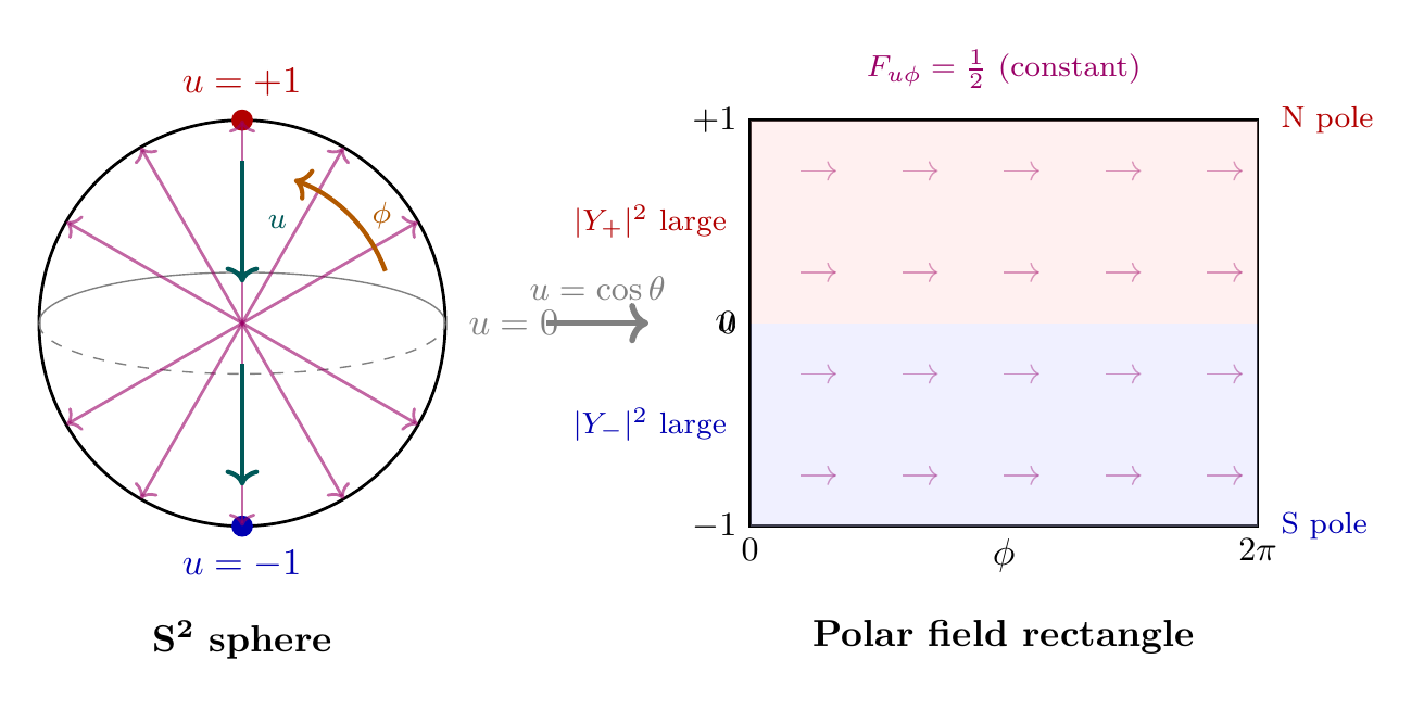
| Field strength | \(F_{\theta\phi} = \frac{1}{2}\sin\theta\) | \(F_{u\phi} = \frac{1}{2}\) (constant) | Is \(F\) position-independent? |
| Coupling factor | \(g^2 \sim 1/\text{Vol}\) | \(g^2 = 4/(3\pi)\) | Does \(3 = 1/\langle u^2\rangle\)? |
| Harmonic norm | \(\int |Y_\pm|^2\sin\theta\,d\theta\) | \(\int (1\pm u)\,du/(4\pi)\) | Linear polynomial? |
In every case, the polar form reveals that TMT quantities are simpler (constant, linear, or polynomial) while classical KK quantities carry Jacobian artifacts (\(\sin\theta\) factors). The “Through vs Around” distinction in the table title above is literally the THROUGH–AROUND decomposition of the polar rectangle \([-1,+1] \times [0,2\pi)\).
Scaffolding note: The polar diagnostic column provides a mechanical check: if a quantity is position-independent or polynomial in \(u\), the TMT interface picture is applicable. If it requires \(\sin\theta\) weighting (position-dependent measure), the classical KK bulk picture is being assumed. This is a coordinate-based test of the physical distinction between surface and volume coupling.
Why the Monopole is Necessary
In TMT, the monopole is not optional. It emerges inevitably from the matching principle.
The Logic:
- Start with the constraint \(ds_6^{\,2} = 0\) (the null condition defining the scaffolding).
- This constraint forces spacetime structure to decompose as \(\mathbb{R}^{1,3} \times S^2\).
- The \(S^2\) factor has non-trivial topology: \(\pi_{2}(S^2) = \mathbb{Z}\).
- Any gauge field configuration on \(S^2\) can wind around the sphere. U(1) bundles are classified by an integer \(n\) (the first Chern class).
- The ground state must have minimal energy. The ground state with nontrivial gauge structure has \(|n| = 1\) (a single monopole).
- This monopole creates a non-trivial \(\text{U(1)}\) bundle, which forces the Higgs field to be a section, not a function.
- Topological obstruction prevents the section from extending to a bulk. Fields are localized on the interface.
- The coupling is now \(g^{2} \sim 0.4\) instead of \(10^{-60}\).
Each step is mathematically rigorous. There is no freedom to avoid the monopole or the topology.
The Matching Relation
The interface principle establishes a precise relationship between the 6D mathematical scaffolding (in which calculations are most elegant) and the 4D observable physics (what we measure).
The Full Matching:
Examples:
- VEV: \(v_{\text{6D}} = 7296 \, \text{GeV} \to v_{\text{obs}} = 246 \, \text{GeV}\) via \(\tau = 1/(3\pi^{2})\)
- Gauge Coupling: \(g_{6}^{2} \sim \text{interface geometry} \to g_{4}^{2} \approx 0.42\) (computed from overlaps)
- Fermion Masses: \(m_{6D} \sim \text{Yukawa overlap on } S^2 \to m_{\text{obs}}\) (matched via VEV scaling)
This matching is the content of what this appendix calls “KK matching” — but it is crucial to emphasize: it is not classical Kaluza-Klein matching. It is the correct matching that accounts for monopole topology and interface physics.
Implications for Theory Choice
The comparison has major implications:
- Classical KK is ruled out: The 60 orders of magnitude discrepancy is not a small correction or a tuning problem. It is a fundamental failure of the model assumptions.
- Extra spatial dimensions (literal): If the universe truly contained literal extra spatial dimensions at the 81 \(\mu\)m scale, they would have been detected long ago by precision tests of gravity and electromagnetism. No such dimensions are observed. Therefore, the \(S^2\) in TMT must not be interpreted as a literal extra dimension.
- The scaffolding interpretation is forced: The \(S^2\) is mathematical scaffolding — a geometric structure used to organize the derivation of 4D physics. The interface principle is the rule for translating between scaffolding quantities and observables.
- TMT is internally consistent: Once the monopole and non-trivial bundle structure are accepted, everything follows with no free parameters (beyond the three input constants \(c, \hbar, G\)).
Open Questions and Future Tests
Several open questions remain, providing targets for future work:
- Experimental Tests: Can we design experiments to probe the 81 \(\mu\)m scale directly? Proposed experiments include precision gravity measurements at sub-mm distances and searches for new fifth-force interactions.
- Neutrino Masses: The absolute neutrino mass scale and mass ordering are predicted by TMT's seesaw mechanism. Neutrinoless double-beta decay experiments can test these.
- CP Violation in Kaons and B Mesons: TMT's CKM and PMNS matrices make specific predictions about CP-violating phases. Rare decay modes probe these.
- Proton Decay: Some unified theories predict proton decay at the \(10^{30}\)-year level. TMT's gauge unification may have implications. Kamiokande and other experiments search for this.
- Fundamental Quantum Decoherence: TMT predicts specific decoherence timescales from Berry phase curvature on \(S^2\). These might be observable in specialized experiments.
—
Summary and Conclusions
This appendix has developed classical Kaluza-Klein theory completely, shown why it fails (60 orders of magnitude), and explained how the interface principle of TMT succeeds by recognizing that monopole topology confines fields to a 2D interface rather than spreading them through a 3D bulk.
Key Results:
- Classical KK: \(g^{2} \sim 10^{-60}\) (disaster)
- Interface: \(g^{2} \approx 0.42\) (observed)
- Difference: Topology (\(\pi_{2}(S^2) = \mathbb{Z}\) forces monopole \(\to\) non-trivial bundle \(\to\) interface localization)
- Polar field coordinates (\(u = \cos\theta\)): transmission coefficient \(\tau = \langle u^2\rangle \times 1/\pi^2\) (THROUGH \(\times\) AROUND), KK tower modes are polynomial \(\times\) Fourier on flat rectangle, monopole field \(F_{u\phi} = 1/2\) constant, spectral zeta decomposes into eigenvalue (THROUGH) and degeneracy (AROUND)
The \(S^2\) is Not a Physical Extra Dimension:
The fact that TMT requires \(S^2\) but predicts no observable extra dimensions (and matches all experiments) means that \(S^2\) must be understood as mathematical scaffolding. It is the framework in which calculations are organized, not a description of additional spatial extent.
Falsifiability:
TMT makes specific predictions that can be tested: the scale \(L_{\xi} \approx 81 \, \mu\text{m}\), the coupling \(g^{2} \approx 0.42\), the fermion mass hierarchy, neutrino properties, and others. If experiments find deviations, TMT is falsified. This is the mark of a scientific theory.
—