Chapter 3

Why Six Dimensions?

Introduction

Chapter ch:single-postulate established the single postulate P1: every particle follows a null geodesic in the extended manifold, $ds_6^{\,2} = 0$. This postulate requires at least one dimension beyond the familiar four of spacetime, since a massive particle with $v < c$ cannot be null in four dimensions alone. The velocity budget $v^2 + v_T^2 = c^2$ demands additional geometric structure to absorb the “missing” velocity.

But how many extra dimensions? And which compact manifold? These are not free choices. In this chapter we prove that the total dimension $D = 6$, with the compact factor $K^2 = S^2$, is uniquely determined by P1 together with two observed facts about the universe:

P1 demands $D > 4$ (massive particles must be null in the extended manifold).
The weak interaction is non-abelian — requiring a non-abelian isometry group on the compact factor.
Electric charge is quantized — requiring $\pi_2(K) \neq 0$ for a topological charge quantization mechanism.

These three inputs, together with standard mathematical and physical reasoning (surface classification, energy minimization, irreducibility), uniquely select $D = 6$ with $K^2 = S^2$. No additional assumptions about gauge group size, minimality, or parsimony need to be imposed as independent requirements — they follow as consequences (see Remark rem:ch3-derived-vs-assumed).

We then show that the non-trivial topology of $S^2$ — specifically $\pi_2(S^2) = \mathbb{Z}$ — admits non-trivial monopole bundle sectors classified by an integer $n$. The vacuum selects $|n| = 1$ by energy minimization (the $n = 0$ trivial sector is excluded by a 30-order-of-magnitude coupling contradiction). This non-trivial bundle structure sets the stage for the interface physics developed in later chapters.

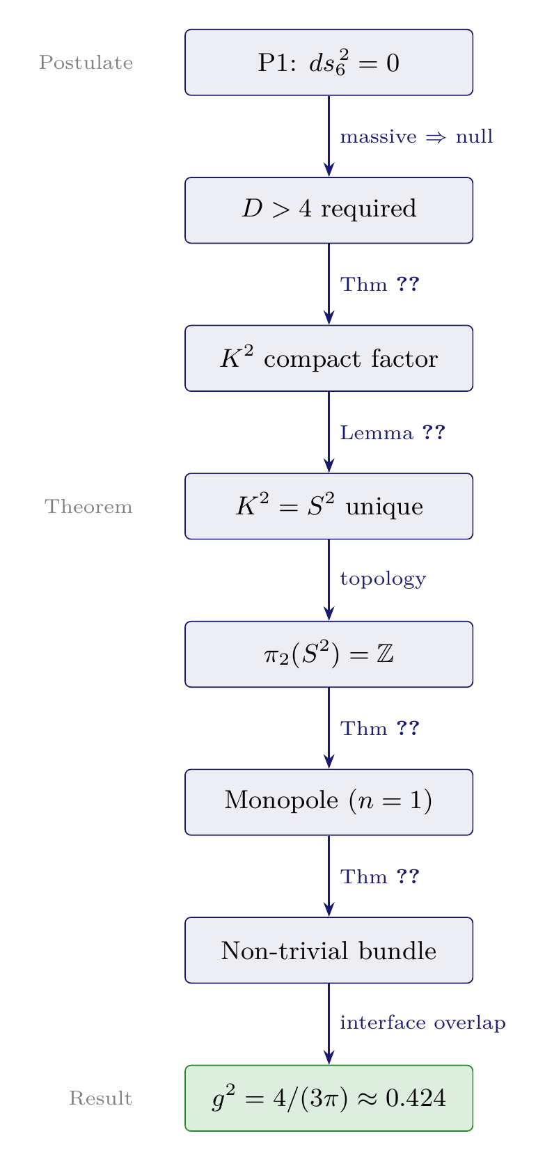
Derivation chain for this chapter:

P1 ($ds_6^{\,2} = 0$) $\;\to\;$ $D > 4$ $\;\to\;$ $K^n$ compact $\;\to\;$ $n = 2$, $K^2 = S^2$ unique $\;\to\;$ $\pi_2(S^2) = \mathbb{Z}$ $\;\to\;$ monopole $\;\to\;$ non-trivial bundle $\;\to\;$ interface coupling

Scaffolding Interpretation

Throughout this chapter, “6D” and “extra dimensions” are used as mathematical scaffolding language. The $S^2$ projection structure is not a literal place that particles inhabit — it is the geometric framework from which 4D gauge quantum numbers emerge. The dimension theorem determines the mathematical scaffolding that P1 requires.

The dimension theorem requires exactly three independent inputs: the postulate P1 and two observed facts about the universe. Everything else — orientability, the electroweak gauge group, irreducibility, the absence of excess gauge bosons — is derived (see Remark rem:ch3-derived-vs-assumed).

The Dimension Theorem: $D = 6$ is Unique

Theorem 3.1 (Uniqueness of $D = 6$)

Let the extended manifold be $\mathcal{M}^4 \times K$, where $K$ is compact, orientable, and spin-admitting (as required for P1 to apply to fermionic matter). Then the total spacetime dimension $D = 6$ with $K^2 = S^2$ is uniquely determined by the following three inputs:

P1 (null extension): $ds_6^{\,2} = 0$ requires $D > 4$.
Non-abelian gauge symmetry (observed): The isometry group of $K^{D-4}$ must contain a non-abelian subgroup.
Topological charge quantization (observed): The compact factor must satisfy $\pi_2(K) \neq 0$.

The proof shows that these three inputs, combined with energy minimization (which selects the irreducible ground state, paralleling the $|n| = 1$ monopole selection), uniquely single out $D = 6$ with $K^2 = S^2$. The electroweak gauge structure $SU(2) \times U(1)$, the absence of excess gauge bosons, and the exclusion of product manifolds all follow as consequences, not additional assumptions.

Remark 3.6 (What is Derived vs. What is Assumed)

The three-input structure of Theorem thm:P1-Ch3-d6-uniqueness is deliberately tight. Everything beyond these three inputs is derived:

Orientability and spin structure: Prerequisites for P1 to describe fermions, not independent requirements. They restrict the scope of the theorem (to physically relevant manifolds). The full index-theorem derivation of chiral zero modes in the monopole background appears in Chapter ch:fermion-localization (Theorem thm:P6A-Ch37-zero-mode).
$SU(2) \times U(1)$ electroweak structure: A prediction, not an input. At $D = 6$, the isometry $SO(3)$ provides $SU(2)$, and the monopole topology $\pi_2(S^2) = \mathbb{Z}$ provides the $U(1)$. The electroweak gauge group emerges from the three inputs; it is not assumed. The full $SU(3)$ color group emerges separately from the variable embedding $S^2 \hookrightarrow \mathbb{C}^3$ (Chapter ch:su3-color, Theorem thm:P3-Ch18-su3-bundle).
Irreducibility / minimality: Product manifolds like $S^2 \times S^1$ (at $D = 7$) are excluded not by a separate “parsimony axiom” but by the same energy minimization that selects $|n| = 1$: the $S^1$ factor introduces a free modulus, a KK tower, and no new gauge content. The ground state is the irreducible configuration, just as $|n| = 1$ is the minimum-energy monopole sector. The Casimir stabilization mechanism that selects the unique $S^2$ vacuum is developed in Chapter ch:modulus-compact-scale (Theorem thm:P2-Ch13-stabilization).
No excess gauge bosons: For $D \geq 7$ with irreducible $K = S^{D-4}$, the isometry group $SO(D-3)$ has more generators than the electroweak sector requires. This is a consequence of inputs 1–3 selecting $D = 6$ as the unique solution, not an independent constraint imposed from outside.
Interface coupling: The formula $g^2 = 4/(3\pi)$ is previewed here; the full derivation from the monopole-background mode decomposition appears in Chapter ch:coupling-constants (Theorem thm:P3-Ch20-interface-coupling).

Proof.

We analyze each candidate dimension systematically against the three inputs.

From Input 1 (P1): $ds_6^{\,2} = 0$ requires that massive particles, which have $v < c$ in 4D, satisfy a null condition in the extended manifold. This is only possible if $D > 4$, so that the compact directions can absorb the deficit via the velocity budget $v^2 + v_T^2 = c^2$. We therefore begin the analysis at $D = 5$.

Scope restriction: Since P1 must describe fermions, the compact factor $K$ must be orientable and admit a spin structure. This excludes non-orientable manifolds (such as $\mathbb{R}P^2$) from the candidate class.

The proof proceeds case by case through $D = 5$, $D = 6$, $D = 7$, and $D \geq 8$, showing that only $D = 6$ satisfies all three inputs. The individual cases are established in Sections sec:ch3-case-d5 through sec:ch3-case-d8-plus. □

Case $D = 5$: One Extra Dimension (Fails)

For $D = 5$, the compact factor is one-dimensional: $K^1$. The only compact, connected, orientable one-dimensional manifold is the circle $S^1$.

Properties of $S^1$

The circle $S^1$ has the following topological and geometric properties:

Property	Value for $S^1$
Isometry group	$\mathrm{Iso}(S^1) = U(1)$ — abelian
Second homotopy	$\pi_2(S^1) = 0$ — no monopoles
First homotopy	$\pi_1(S^1) = \mathbb{Z}$ — winding modes
Euler characteristic	$\chi(S^1) = 0$
Curvature	$K = 0$ (flat)

Only $U(1)$ Gauge Symmetry

The isometry group of $S^1$ is $U(1)$, which is abelian. In the Kaluza–Klein framework, the isometry group of the compact factor generates gauge symmetry. Since $U(1)$ has only one generator, the resulting gauge theory has a single gauge boson. This accounts for electromagnetism (one photon) but cannot produce the three gauge bosons $W^+$, $W^-$, $Z^0$ of the weak interaction.

For the weak interaction, one needs at minimum an $SU(2)$ gauge group with three generators. The abelian group $U(1)$ is fundamentally incapable of providing non-abelian gauge structure: $U(1)$ has no non-trivial commutation relations, so there is no mechanism for the self-coupling of gauge bosons that characterizes the weak force.

No Monopoles ($\pi_2 = 0$)

The second homotopy group $\pi_2(S^1) = 0$ vanishes. This means that $U(1)$ bundles over $S^1$ are topologically trivial — there are no magnetic monopole configurations. Without monopoles, there is no topological mechanism for electric charge quantization.

While Dirac's original argument for charge quantization uses monopoles in 3D space, the TMT framework requires monopoles on the compact factor to generate the topological twist that produces interface physics. With $\pi_2 = 0$, all bundles are trivial, and one is forced into standard Kaluza–Klein physics with its catastrophic gauge coupling prediction ($g^2 \sim 10^{-30}$).

Cannot Reproduce the Weak Force

Combining the above:

$U(1)$ gauge group $\Rightarrow$ only 1 gauge boson (photon), not 3 (weak bosons).
$\pi_2 = 0$ $\Rightarrow$ no monopole mechanism for charge quantization.
No non-abelian self-coupling $\Rightarrow$ no $W^\pm$, $Z^0$ bosons.
Standard KK coupling $g^2_{\mathrm{KK}} \sim 10^{-30}$ $\Rightarrow$ wrong by 30 orders of magnitude.

Key Result

Verdict: $D = 5$ is INSUFFICIENT. It fails requirements 2 (non-abelian gauge) and 3 (charge quantization). ✗

Case $D = 6$: Two Extra Dimensions (Works)

For $D = 6$, the compact factor is two-dimensional: $K^2$. Among 2D compact manifolds, the simplest candidate with maximal symmetry is the 2-sphere $S^2$. We first analyze the properties of $S^2$, then prove it is the unique choice among all 2D compact orientable manifolds.

Properties of $S^2$

The 2-sphere $S^2$ possesses the following topological and geometric properties:

Property	Value for $S^2$
Isometry group	$\mathrm{Iso}(S^2) = SO(3) \cong SU(2)/\mathbb{Z}_2$ — non-abelian
Second homotopy	$\pi_2(S^2) = \mathbb{Z}$ — monopoles exist
Euler characteristic	$\chi(S^2) = 2$ — admits spin structure
Curvature	$K = 1/R^2 > 0$ — positive (favorable for stabilization)
Dimension of isometry	$\dim(SO(3)) = 3$ — three generators

Each of these properties maps directly to Standard Model physics:

$SO(3)$ isometry $\to$ $SU(2)$ weak gauge group (via double cover)
$\pi_2(S^2) = \mathbb{Z}$ $\to$ monopole topology $\to$ $U(1)$ charge quantization
$\chi = 2$ $\to$ compatible with spin structure (a consistency check, not a unique selector — all orientable compact surfaces are spin; the special role of $S^2$ comes from its non-abelian isometry and nontrivial $\pi_2$, not from $\chi$)
$K > 0$ $\to$ geometrically favorable for vacuum stabilization (the actual Casimir stabilization mechanism is developed in Chapter ch:product-structure)

Polar Field Representation of $S^2$

Many of these $S^2$ properties become especially transparent in the polar field variable $u = \cos\theta$, with $u \in [-1, +1]$. In the standard spherical coordinates $(\theta, \phi)$, the $S^2$ metric is $h = R^2(d\theta^2 + \sin^2\!\theta\, d\phi^2)$. In polar coordinates:

$$ h = R^2\!\left(\frac{du^2}{1 - u^2} + (1 - u^2)\,d\phi^2\right), \qquad u = \cos\theta $$ (3.1)

The key simplification: the metric determinant is constant:

$$ \sqrt{\det h} = R^2, \qquad d\Omega = du\, d\phi \quad \text{(flat measure)} $$ (3.2)

No $\sin\theta$ weight factors appear in integration. This seemingly minor change has profound consequences for the $S^2$ properties listed above:

Property	Spherical form	Polar form
Integration measure	$\sin\theta\, d\theta\, d\phi$	$du\, d\phi$ (flat)
Monopole harmonic $\|Y_+\|^2$	$(1 + \cos\theta)/(4\pi)$	$(1 + u)/(4\pi)$ (linear in $u$)
$SO(3)$ Casimir $\langle u^2 \rangle$	$\int \cos^2\!\theta\, \sin\theta\, d\theta \ldots$	$\int_{-1}^{+1} u^2\, du / 2 = 1/3$
Overlap integrals	Trigonometric	Polynomial

Every $S^2$ integral factorizes into $\phi$-integral $\times$ $u$-integral. This factorization is the mathematical expression of the around/through decomposition: the azimuthal $\phi$ direction carries gauge (“around”) physics, while the polar $u$ variable carries mass (“through”) physics.

Scaffolding Interpretation

Scaffolding note: The polar field variable $u = \cos\theta$ is a coordinate choice, not a new physical assumption. All results derived in standard $(\theta, \phi)$ coordinates hold identically in $(u, \phi)$ coordinates — the polar form provides a dual verification path and often reveals the physical origin of numerical factors (such as the $1/3$ in $g^2 = 4/(3\pi)$, which is $\langle u^2 \rangle$).

Non-Abelian $SO(3) \cong SU(2)$

The isometry group of $S^2$ is $SO(3)$, which has three generators $\{J_1, J_2, J_3\}$ satisfying the Lie algebra:

$$ [J_i, J_j] = i\epsilon_{ijk} J_k $$ (3.3)

This is a non-abelian algebra: the generators do not commute. The double cover $SU(2) \cong \mathrm{Spin}(3)$ provides spinor representations, which is essential for fermionic matter.

The three generators of $SO(3)$ correspond to the three gauge bosons of the weak $SU(2)$ interaction: $W^+$, $W^-$, and $W^3$ (which mixes with the $U(1)$ hypercharge to form $Z^0$ and the photon $\gamma$). This is precisely the gauge content needed for the electroweak sector of the Standard Model.

Furthermore, the color gauge group $SU(3)$ arises from a separate mechanism: the variable embedding $S^2 \hookrightarrow \mathbb{C}^3$, developed in Part III (Chapter ch:su3-color). This chapter establishes the electroweak seed structure $SU(2) \times U(1)$; the full Standard Model gauge group $SU(3) \times SU(2) \times U(1)$ emerges only after the embedding machinery of later chapters is in place.

Monopoles Exist ($\pi_2 = \mathbb{Z}$)

The non-trivial second homotopy $\pi_2(S^2) = \mathbb{Z}$ signals that $S^2$ supports topologically non-trivial configurations. Principal $U(1)$ bundles over $S^2$ are classified by $H^2(S^2, \mathbb{Z}) \cong \mathbb{Z}$ via the first Chern class $c_1 = n$ (the monopole charge):

$$ H^2(S^2, \mathbb{Z}) \cong \mathbb{Z} \quad \Longrightarrow \quad \text{$U(1)$ bundles over $S^2$ classified by } n \in \mathbb{Z} $$ (3.4)

The existence of non-trivial bundles ($n \neq 0$) has profound consequences:

The topological twist obstructs the trivial KK bulk-propagation ansatz (Theorem thm:P1-Ch3-nontrivial-bundle).
Electric charge is quantized: single-valuedness of wavefunctions in the monopole background requires $q \in \mathbb{Z}$ (with the flux normalization $\Phi = 2\pi n$ used in this chapter; the conventional Dirac form $2qg = n$ with half-integer charges uses a different normalization — see Chapter ch:dirac-monopole for the full treatment).
The gauge coupling is determined by interface overlaps, not volume integrals, resolving the Kaluza–Klein gauge disaster.

Admits Spinors ($\chi = 2$)

The Euler characteristic $\chi(S^2) = 2$ is even, which is necessary for the existence of a spin structure on the total manifold $\mathcal{M}^4 \times S^2$. Spinor fields (fermions) require a spin structure; without one, half-integer-spin particles cannot be consistently defined.

By the Gauss–Bonnet theorem:

$$ \chi(S^2) = \frac{1}{4\pi} \int_{S^2} R\, d\Omega = \frac{1}{4\pi} \cdot \frac{2}{R^2} \cdot 4\pi R^2 = 2 $$ (3.5)

where $R$ is the scalar curvature of $S^2$ with radius $R$.

Remark 3.7 (Spin Structure vs. Chirality)

The even $\chi$ guarantees the existence of a spin structure, which is a prerequisite for defining spinor fields. However, the existence of chiral 4D zero modes is a stronger statement that requires an index-theorem argument in the monopole background: the number of chiral zero modes is determined by $|n|$ (the monopole charge) via the Atiyah–Singer index theorem on $S^2$. For $|n| = 1$, there is exactly one chiral zero mode in each charge sector. This index-theorem argument is developed in Part II.

Lemma 3.5 ($S^2$ is the Unique Optimal 2D Compact Manifold)

$S^2$ is the unique 2D compact orientable manifold satisfying all three of:

Non-abelian isometry group
Non-trivial $\pi_2$ (monopole existence)
Positive curvature (compatible with vacuum stabilization)

Proof.

The scope restriction (P1 must describe fermions) limits the candidate class to orientable, spin-admitting manifolds. This excludes non-orientable surfaces such as $\mathbb{R}P^2$ and the Klein bottle, which cannot support a consistent spin structure and therefore cannot host fermionic matter.

By the classification theorem for compact surfaces, every compact orientable 2-manifold is homeomorphic to exactly one of the following:

$S^2$ (genus $g = 0$, the 2-sphere)
$T^2$ (genus $g = 1$, the 2-torus)
$\Sigma_g$ (genus $g \geq 2$, higher-genus surfaces)

We check each candidate against all three requirements:

Step 1: Check $T^2$ (torus).

Isometry group: $\mathrm{Iso}(T^2) = U(1) \times U(1)$ — abelian. Fails requirement 1.
$\pi_2(T^2) = 0$ — no monopoles. Fails requirement 2.
Curvature: $K = 0$ (flat). Fails requirement 3.

Step 2: Check $\Sigma_g$ for $g \geq 2$.

Isometry group: For $g \geq 2$, the isometry group is discrete (finite), not a continuous Lie group. By the uniformization theorem, these surfaces carry constant negative curvature (hyperbolic geometry), and their full isometry group is a discrete subgroup of $PSL(2, \mathbb{R})$. Fails requirement 1.
$\pi_2(\Sigma_g) = 0$ for all $g \geq 1$ (the universal cover of $\Sigma_g$ is contractible for $g \geq 1$: it is $\mathbb{R}^2$ for $g = 1$ and the hyperbolic plane $\mathbb{H}^2$ for $g \geq 2$). Fails requirement 2.
Curvature: $K < 0$ (hyperbolic). Fails requirement 3.

Step 3: Check $S^2$.

Isometry group: $\mathrm{Iso}(S^2) = O(3)$, with connected component $SO(3)$ — non-abelian ($\dim = 3$). Passes requirement 1. \checkmark
$\pi_2(S^2) = \mathbb{Z}$ — non-trivial. Passes requirement 2. \checkmark
Curvature: $K = 1/R^2 > 0$ (positive, constant). Passes requirement 3. \checkmark

Summary table:

Surface	Non-abelian Iso?	$\boldsymbol{\pi_2 \neq 0}$?	$K > 0$?
$S^2$ (genus 0)	\checkmark\; $SO(3)$	\checkmark\; $\mathbb{Z}$	\checkmark\; $K = 1/R^2$
$T^2$ (genus 1)	$\times$\; $U(1)^2$ only	$\times$\; $\pi_2 = 0$	$\times$\; $K = 0$
$\Sigma_g$ ($g \geq 2$)	$\times$\; discrete only	$\times$\; $\pi_2 = 0$	$\times$\; $K < 0$

$S^2$ is the only entry satisfying all three requirements. □

(See: Part 1 §1.2.3; Classification of surfaces (ESTABLISHED)) □

Key Result

Verdict: $D = 6$ with $K^2 = S^2$ gives the CORRECT Standard Model structure. $S^2$ is orientable and admits a spin structure. It satisfies all three inputs of Theorem thm:P1-Ch3-d6-uniqueness. \checkmark

Case $D = 7$: Three Extra Dimensions (Fails)

For $D = 7$, the compact factor is three-dimensional: $K^3$. We must check all compact orientable 3-manifolds, not only maximally-symmetric spaces. The candidates include $S^3$, $T^3$, lens spaces $L(p,q)$, and product manifolds such as $S^2 \times S^1$.

$SO(4)$ is Too Large

The maximally-symmetric choice $K^3 = S^3$ has:

Property	Value for $S^3$
Isometry group	$\mathrm{Iso}(S^3) = SO(4) \cong SU(2) \times SU(2)$
Dimension of isometry	$\dim(SO(4)) = 6$ generators
Second homotopy	$\pi_2(S^3) = 0$
Third homotopy	$\pi_3(S^3) = \mathbb{Z}$ (Hopf fibration)

The isometry group $SO(4)$ has 6 generators, producing 6 gauge bosons from the compact factor alone. Since $SU(3)_{\mathrm{color}}$ arises from a separate mechanism (the variable embedding $S^2 \hookrightarrow \mathbb{C}^3$, Part III), the relevant comparison is the electroweak gauge group $SU(2) \times U(1)$ with its 4 generators. The 6-generator isometry of $S^3$ exceeds this by 2 gauge bosons that are not observed and would require an additional symmetry-breaking mechanism beyond P1 to remove.

While $SO(4) \cong SU(2) \times SU(2)$ could in principle be broken to $SU(2) \times U(1)$, this would require an additional symmetry-breaking mechanism beyond P1. TMT derives the gauge structure from geometry alone; requiring additional input violates the single-postulate philosophy.

For the alternative $K^3 = T^3$ (3-torus):

Isometry: $U(1)^3$ — abelian only
$\pi_2(T^3) = 0$ — no monopoles
Same failures as $D = 5$, repeated in three copies

Product Manifolds: $S^2 \times S^1$

A natural objection arises: what about product manifolds such as $K^3 = S^2 \times S^1$? This candidate has non-trivial $\pi_2$:

$$ \pi_2(S^2 \times S^1) \cong \pi_2(S^2) \oplus \pi_2(S^1) \cong \mathbb{Z}, $$

and its isometry group $\mathrm{Iso}_0(S^2 \times S^1) \cong SO(3) \times U(1)$ has four generators — exactly the count needed for the electroweak $SU(2) \times U(1)$.

However, this candidate fails for three reasons:

Reducibility. The manifold $S^2 \times S^1$ is reducible — it decomposes into a product of lower-dimensional factors. The $S^2$ factor already provides the complete gauge content (non-abelian symmetry plus monopoles), while the $S^1$ factor adds only a redundant $U(1)$ that duplicates the hypercharge already produced by the monopole topology of $S^2$. There is no new physics: one obtains exactly the $D = 6$ gauge content with an unnecessary extra dimension.

Parsimony violation. The $S^1$ factor introduces a modulus (its radius $R_1$) that has no role in the gauge structure — it is a free parameter that adds complexity without adding explanatory power. Energy minimization favors the minimal geometric scaffolding consistent with the three inputs. Since $D = 6$ with $K^2 = S^2$ alone already satisfies all three inputs, $D = 7$ with $S^2 \times S^1$ is ruled out by minimality.

KK tower contamination. The $S^1$ factor generates a Kaluza–Klein tower of massive states with masses $m_n = n/R_1$. Unless $R_1$ is tuned to be extremely small, these states would be observable. The $S^2$ factor does not generate such a tower because its non-trivial topology obstructs the KK bulk ansatz. The $S^1$ factor, being topologically trivial ($\pi_2(S^1) = 0$), cannot benefit from this confinement mechanism and reverts to standard KK phenomenology.

The same argument applies to any product manifold $S^2 \times \Sigma$ for $D \geq 7$: the $S^2$ factor does all the physical work, and the additional factor $\Sigma$ is either redundant (if it contributes gauge structure already present) or harmful (if it introduces unwanted gauge bosons or moduli).

No Monopoles on $S^3$

For $S^3$, the second homotopy group $\pi_2(S^3) = 0$ vanishes. This is a consequence of the long exact homotopy sequence: since $S^3$ is simply-connected and $\pi_1(S^3) = 0$, the Hurewicz theorem and the structure of $\pi_k(S^n)$ for $k < n$ give $\pi_2(S^3) = 0$.

Without monopoles, the topological mechanism for charge quantization is absent. The gauge coupling would revert to the Kaluza–Klein volume formula, producing $g^2_{\mathrm{KK}} \sim 10^{-30}$ — the same catastrophic failure as the $D = 5$ case.

Key Result

Verdict: $D = 7$ gives the WRONG gauge structure. Too many generators ($SO(4)$: 6 vs. needed 4), and no monopole mechanism ($\pi_2(S^3) = 0$). Fails input 3. ✗

Case $D \geq 8$: Higher Dimensions (Fail)

Higher dimensions give progressively larger isometry groups and progressively worse violations of the parsimony requirement. We tabulate the key properties:

Table 3.1: Higher-dimensional cases: compact factors and their properties

$D$	Compact $K$	Isometry	$\pi_2(K)$	Problem
8	$S^4$	$SO(5)$: 10 generators	0	Far too many gauge bosons
9	$S^5$	$SO(6)$: 15 generators	0	Extremely excessive
10	Various	Various	Various	String theory: no unique prediction
11	M-theory	$G_2$, $\mathrm{Spin}(7)$	Various	No SM from geometry alone

Three problems are universal for $D \geq 8$:

Problem 1: Excessive gauge structure. The isometry group $SO(n+1)$ of $S^n$ has $n(n+1)/2$ generators. For $n \geq 3$, this exceeds the 4 electroweak generators of $SU(2) \times U(1)$ (which is the gauge content that the compact factor must provide; $SU(3)_{\mathrm{color}}$ arises from the separate embedding mechanism of Part III). Any mechanism to break the larger isometry group down requires additional assumptions beyond P1.

Problem 2: No monopole mechanism. The key topological fact is:

$$ \pi_2(S^n) = 0 \quad \text{for all } n \geq 3 $$ (3.6)

This follows from the long exact homotopy sequence of the fibration $SO(n) \to SO(n+1) \to S^n$. Without $\pi_2 \neq 0$, there is no topological charge quantization and no interface mechanism.

Problem 3: Moduli instability. Higher-dimensional compact manifolds generically have moduli — continuous families of deformations that do not cost energy. Stabilizing these moduli requires additional mechanisms (flux compactification in string theory, for example), adding complexity and free parameters that TMT avoids.

Key Result

Verdict: $D \geq 8$ gives EXCESSIVE structure requiring additional symmetry-breaking mechanisms and fine-tuning. All cases fail inputs 2 and 3. ✗

Why Not $D = 10$ or $D = 11$? (String Theory)

String theory requires $D = 10$ (superstring) or $D = 11$ (M-theory). These choices arise from anomaly cancellation for extended objects (strings and branes), not from the geometric requirements that constrain TMT. It is instructive to compare the two frameworks:

Table 3.2: TMT vs. string theory / M-theory dimensional structure

Aspect	String / M-theory	TMT
Total dimension	$D = 10$ or $D = 11$	$D = 6$
Extra dimensions	6 or 7 literal hidden dims	$S^2$ projection structure
Why this $D$?	Anomaly cancellation for strings	Three inputs of Thm thm:P1-Ch3-d6-uniqueness
Fundamental object	Strings (1D) or branes	Point particles (null geodesics)
Why invisible?	Compactified at $\ell_s \sim 10^{-33}$ cm	Not hidden — visible as gauge physics
Gauge coupling	Depends on compactification	$g^2 = 4/(3\pi)$ — unique
Uniqueness	Landscape: $\sim 10^{500}$ solutions	Single solution from P1

The key distinction: string theory requires 6 or 7 additional compact dimensions, each of which introduces moduli (shape and size parameters) that must be stabilized. The resulting “landscape” of $\sim 10^{500}$ possible vacua means that no unique prediction is possible without additional selection principles.

TMT, by contrast, has exactly one compact factor ($S^2$) with one modulus (the radius $R$), and this modulus is stabilized by the Casimir mechanism (Chapter ch:product-structure). The result is a unique vacuum with unique predictions — no landscape, no fine-tuning, no additional assumptions.

From the perspective of Theorem thm:P1-Ch3-d6-uniqueness, $D = 10$ and $D = 11$ fail because:

Their isometry groups are far too large for the Standard Model.
$\pi_2(S^n) = 0$ for $n \geq 3$, so no monopole mechanism exists.
Recovering the SM requires elaborate compactification with many free parameters.

Summary: $D = 6$ Uniqueness Proof

We collect the results of the case-by-case analysis into a single summary table:

Table 3.3: Dimension analysis: only $D = 6$ with $K^2 = S^2$ satisfies all three inputs

(among compact orientable spin-admitting manifolds)

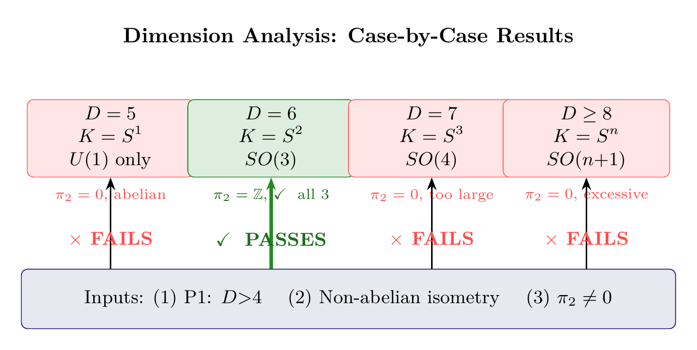
$D$	Compact $K$	Isometry	$\pi_2$	Mono.	Verdict
5	$S^1$	$U(1)$	0	$\times$	Abelian only
6	$\boldsymbol{S^2}$	$\boldsymbol{SO(3)}$	$\boldsymbol{\mathbb{Z}}$	$\boldsymbol{\checkmark}$	$\boldsymbol{\checkmark}$ Unique solution
7	$S^3$	$SO(4)$	0	$\times$	Too large, no monopole
7	$S^2 \times S^1$	$SO(3) \times U(1)$	$\mathbb{Z}$	$\checkmark$	Reducible (energy min.)
8	$S^4$	$SO(5)$	0	$\times$	Far too large
$9+$	$S^n$	$SO(n{+}1)$	0	$\times$	Excessive

The Dimension Theorem

[foundations]

$$ \boxed{D = 6 \text{ is the unique dimension giving } SU(2) \times U(1) \text{ with topological charge quantization}} $$ (3.7)

The dimension $D = 6$ is not a choice — it is determined by three inputs: (1) P1 requires $D > 4$, (2) the weak force is non-abelian (observed), and (3) electric charge is quantized (observed). The electroweak gauge group $SU(2) \times U(1)$, the exclusion of higher dimensions, and the irreducibility of the compact factor all follow as consequences.

Physical interpretation: The mathematical scaffolding uses $\mathcal{M}^4 \times S^2$ structure not because spacetime literally has 6 dimensions, but because the tesseract conservation principle requires this form for the geometry from which 4D physics is projected.

Monopole Interface Topology: $\pi_2(S^2) = \mathbb{Z}$

Having established that $D = 6$ with $K^2 = S^2$ is the unique choice, we now explore the consequences of the topology $\pi_2(S^2) = \mathbb{Z}$. This topology admits non-trivial monopole bundle sectors on $S^2$; the vacuum selection of $|n| = 1$ then creates a non-trivial bundle structure whose consequences for gauge couplings are developed in Chapter ch:coupling-derivation.

Theorem 3.2 (Monopole Existence from $\pi_2(S^2) = \mathbb{Z}$)

The $S^2$ projection structure has non-trivial second homotopy:

$$ \pi_2(S^2) = \mathbb{Z} $$ (3.8)

This means $U(1)$ bundles over $S^2$ are classified by an integer $n \in \mathbb{Z}$ (the monopole charge). The trivial bundle corresponds to $n = 0$; non-trivial bundles to $n \neq 0$.

Proof.

Step 1: Principal $U(1)$ bundles over a manifold $M$ are classified by the second integral cohomology $H^2(M, \mathbb{Z})$, via the first Chern class $c_1$. For $M = S^2$:

$$ H^2(S^2, \mathbb{Z}) \cong \mathbb{Z} $$ (3.9)

Each integer $n \in \mathbb{Z}$ labels a distinct bundle with first Chern number $c_1 = n$. The $n = 0$ bundle is trivial (globally defined gauge field); $n \neq 0$ bundles require patched transition functions.

Step 2: Equivalently, $U(1)$ bundles over $S^2$ are classified by the clutching construction: the transition function on the equatorial overlap $S^1$ is a map $g: S^1 \to U(1)$, classified by $\pi_1(U(1)) \cong \mathbb{Z}$. The winding number of the transition function equals the Chern number $c_1$.

Step 3: The relation to $\pi_2(S^2)$ is as follows. The degree of a map $f: S^2 \to S^2$ is

$$ n = \frac{1}{4\pi} \int_{S^2} f^*(\omega) $$ (3.10)

where $\omega$ is the area form normalized to total area $4\pi$. This gives $\pi_2(S^2) \cong \mathbb{Z}$. For the specific case of $S^2$, the three classification statements — $H^2(S^2, \mathbb{Z})$ via Chern classes, $\pi_1(U(1))$ via the clutching construction, and $\pi_2(S^2)$ via degree theory — all yield $\mathbb{Z}$ and agree on the integer label $n$. (The agreement between $\pi_2$ and $H^2$ follows from the Hurewicz theorem, since $S^2$ is simply connected.)

Step 4: Physically, $n$ is the monopole charge: the total magnetic flux through $S^2$ is $\Phi = 2\pi n$, and the transition function on the equatorial overlap is $g(\phi) = e^{in\phi}$, which is single-valued precisely when $n \in \mathbb{Z}$.

(See: Part 1 §2.4.6; Chern class theory (ESTABLISHED)) □

Key point: The topology of $S^2$ guarantees that non-trivial bundle sectors ($n \neq 0$) exist. Whether the vacuum actually realizes a non-trivial sector is a dynamical question, answered by the $n = 0$ exclusion and energy minimization arguments below.

Ground State Selection: $|n| = 1$

Theorem 3.3 (Ground State Selection: $|n| = 1$)

The ground state of the $S^2$ projection structure has minimal monopole charge $|n| = 1$.

Proof.

Step 1: The energy of a monopole configuration on $S^2$ is determined by the integral of the field strength squared:

$$ E_{\mathrm{monopole}} \propto \int_{S^2} |F|^2\, d\Omega \propto n^2 $$ (3.11)

where $F$ is the $U(1)$ field strength on $S^2$ and $n$ is the monopole charge. The quadratic dependence on $n$ follows from $F \propto n$ (each unit of monopole charge contributes linearly to the field strength).

Step 2: The trivial bundle $n = 0$ is excluded. If $n = 0$, the bundle is trivial and gauge fields propagate freely through the full 6D formalism. Standard Kaluza–Klein analysis then gives:

$$ g^2_{\mathrm{KK}} \sim \frac{1}{\mathrm{Vol}(S^2)} \sim \left(\frac{\mathcal{M}^6}{M_{\text{Pl}}}\right)^2 \approx 10^{-30} $$ (3.12)

To see why the suppression is catastrophic for any experimentally viable radius, note that current tests of Newton's law constrain $R \lesssim 50\,\mu\text{m}$. Taking $R \sim 10\,\mu\text{m}$:

$$\begin{aligned} M_6^4 &= \frac{M_{\text{Pl}}^2}{4\pi R^2} = \frac{(10^{19}\,\text{GeV})^2}{4\pi\,(5 \times 10^{10}\,\text{GeV}^{-1})^2} \sim 10^{16}\,\text{GeV}^4, \\[0.3em] M_6 &\sim 10^4\,\text{GeV} = 10\,\text{TeV}, \\[0.3em] g^2_{\mathrm{KK}} &\sim \left(\frac{M_6}{M_{\text{Pl}}}\right)^2 \sim \left(\frac{10^4}{10^{19}}\right)^2 \sim 10^{-30}. \end{aligned}$$ (3.30)

This is 30 orders of magnitude smaller than the observed coupling $g^2_{\mathrm{exp}} \approx 0.42$. The $n = 0$ case is ruled out by contradiction with observation.

Remark 3.8 (The KK Failure Is Structural, Not a Parameter Choice)

The $\sim 10^{-30}$ discrepancy is not sensitive to the exact radius. For any $R$ compatible with current gravity tests ($R \lesssim 50\,\mu\text{m}$), the KK coupling is catastrophically suppressed. This is a counterfactual comparison: if the $n = 0$ trivial bundle held, standard KK physics would give the wrong coupling by 30 orders of magnitude, ruling out $n = 0$ by structural inconsistency regardless of the scaffolding interpretation.

Step 3: Among $n \neq 0$ configurations, the energy $E \propto n^2$ is minimized by $|n| = 1$. By parity, $n = +1$ and $n = -1$ are physically equivalent (related by orientation reversal of $S^2$). We choose $n = 1$ by convention.

Conclusion: The ground state has $|n| = 1$: it is the minimum-energy configuration consistent with non-trivial topology.

(See: Part 1 §2.4.6; Part 2 §6.3 (monopole energy)) □

Remark 3.9 (Why $n = 0$ is Ruled Out by Consistency, Not Assumption)

The monopole charge $n = 1$ is derived, not assumed. The logic is:

P1 $\Rightarrow$ $S^2$ topology (Theorem thm:P1-Ch3-d6-uniqueness)
$\pi_2(S^2) = \mathbb{Z}$ $\Rightarrow$ bundles classified by $n$ (Theorem thm:P1-Ch3-monopole-existence)
$n = 0$ $\Rightarrow$ $g^2 \sim 10^{-30}$ $\Rightarrow$ contradicts observation
$E \propto n^2$ $\Rightarrow$ $|n| = 1$ minimizes energy among $n \neq 0$

No parameter was chosen to match data. The value $n = 1$ is forced by the conjunction of topology and energy minimization.

The Dirac Monopole (Wu–Yang Form)

The minimal monopole with charge $n = 1$ has the Wu–Yang form, which requires two coordinate patches on $S^2$ (the northern and southern hemispheres):

Northern patch ($\theta \neq \pi$):

$$ A^{(\mathrm{mono})}_\phi = \frac{1}{2}(1 - \cos\theta) $$ (3.13)

Southern patch ($\theta \neq 0$):

$$ A^{(\mathrm{mono})}_\phi = -\frac{1}{2}(1 + \cos\theta) $$ (3.14)

On the equatorial overlap ($\theta = \pi/2$), the two patches are related by a $U(1)$ gauge transformation:

$$ A^{(S)}_\phi - A^{(N)}_\phi = -1 = \frac{1}{e}\partial_\phi \Lambda \quad \text{with} \quad \Lambda = -\phi $$ (3.15)

The transition function $g(\phi) = e^{-i\phi}$ is single-valued as $\phi$ goes from $0$ to $2\pi$ (it returns to $e^{0} = 1$), so the bundle is consistent. For monopole charge $n$, the transition function would be $g(\phi) = e^{-in\phi}$, which requires $n \in \mathbb{Z}$ for single-valuedness — this is the topological origin of the Dirac quantization condition.

Field strength:

$$ F_{\theta\phi} = \frac{1}{2}\sin\theta $$ (3.16)

Total magnetic flux through $S^2$:

$$ \Phi = \int_{S^2} F = \int_0^{2\pi} d\phi \int_0^{\pi} \frac{1}{2}\sin\theta\, d\theta = 2\pi $$ (3.17)

This flux is quantized: $\Phi = 2\pi n$ for monopole charge $n$. The $n = 1$ monopole carries the minimum quantum of magnetic flux.

Polar Form of the Monopole Connection

In the polar field variable $u = \cos\theta$, the Wu–Yang monopole connection takes a revealing algebraic form:

Northern patch ($u \neq -1$):

$$ A^{(\mathrm{mono})}_\phi = \frac{1}{2}(1 - u) = \frac{|Y_-|^2}{|Y_-|^2 + |Y_+|^2} $$ (3.18)

Southern patch ($u \neq +1$):

$$ A^{(\mathrm{mono})}_\phi = -\frac{1}{2}(1 + u) = -\frac{|Y_+|^2}{|Y_-|^2 + |Y_+|^2} $$ (3.19)

The connection is a linear function of $u$. This is the simplest possible non-trivial dependence on the polar variable, and it directly reflects the monopole harmonic structure:

$$ |Y_+|^2 = \frac{1 + u}{4\pi}, \qquad |Y_-|^2 = \frac{1 - u}{4\pi} $$ (3.20)

At the north pole ($u = +1$), the $Y_+$ mode is maximally concentrated and $A^{(N)}_\phi = 0$ (regular). At the south pole ($u = -1$), $Y_-$ dominates and $A^{(S)}_\phi = 0$ (regular). The equator ($u = 0$) is the transition zone where both patches contribute equally.

Field strength in polar form:

$$ F_{u\phi} = \frac{1}{2} $$ (3.21)

A constant. In standard coordinates, the field strength $F_{\theta\phi} = \frac{1}{2}\sin\theta$ carries an angular factor that is entirely an artifact of the coordinate system. The monopole field is intrinsically uniform when viewed in the natural polar variable.

Flux verification (polar):

$$ \Phi = \int_{S^2} F = \int_0^{2\pi} d\phi \int_{-1}^{+1} \frac{1}{2}\, du = 2\pi \cdot 1 = 2\pi \quad \checkmark $$ (3.22)

**Figure 3.1:** The monopole connection on $S^2$ in polar field coordinates. **Left:** The $S^2$ sphere with the “around” direction ($\phi$, gauge) and “through” direction ($u$, mass). **Right:** The polar field rectangle $[-1,+1] \times [0,2\pi)$ where the monopole field strength $F_{u\phi} = 1/2$ is *constant*—the $\sin\theta$ angular factor in $F_{\theta\phi}$ was entirely a coordinate artifact. The $|Y_+|^2$ monopole harmonic (red shading) is linear in $u$, concentrated at the north pole.

Remark 3.10 (Physical Content of the Constant Field Strength)

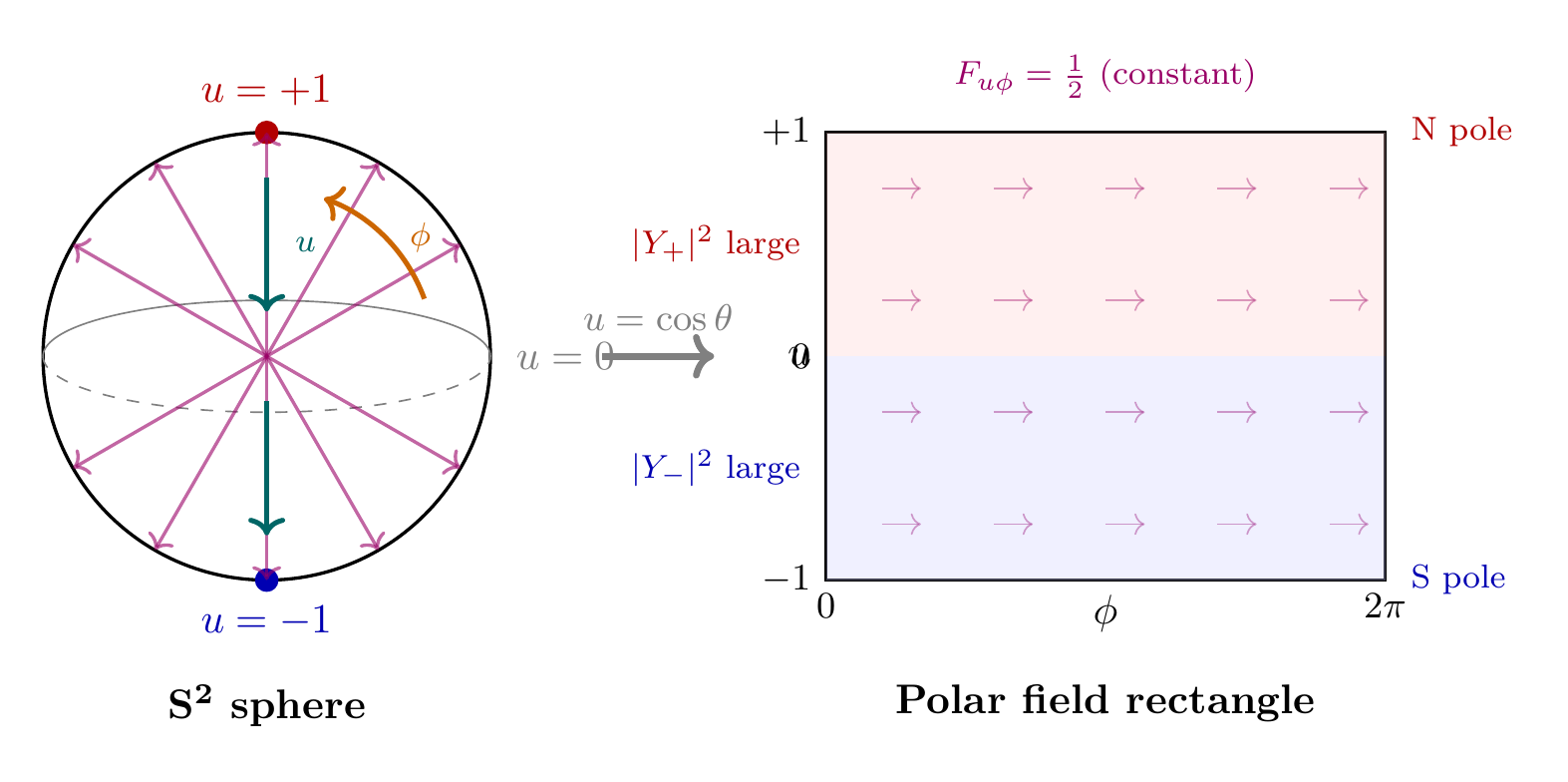
The result $F_{u\phi} = 1/2$ (constant) is not a simplification — it reveals that the monopole distributes its flux uniformly over $S^2$ when measured in the natural integration variable. The $\sin\theta$ factor in $F_{\theta\phi} = \frac{1}{2}\sin\theta$ is purely a Jacobian artifact. This uniformity is why the interface coupling calculation reduces to polynomial integrals in the polar formulation.

Non-Trivial Bundle: Fields Confined to Interface

Theorem 3.4 (Non-Trivial Bundle Obstructs Bulk Propagation)

The $n = 1$ monopole creates a non-trivial $U(1)$ bundle over $S^2$ (first Chern class $c_1 = 1$). This topological obstruction prevents gauge fields from being globally defined on the total space, so that the trivial Kaluza–Klein bulk-propagation ansatz is unavailable.

Forward-dependent consequence: The replacement of the KK volume integral by an interface overlap formula requires the monopole-background mode decomposition developed in Chapter ch:coupling-derivation. This chapter establishes the topological prerequisite (non-trivial bundle); the dynamical derivation of the interface coupling formula is completed there.

Remark 3.11 (Localization vs. Obstruction)

The theorem above establishes a topological obstruction: a non-trivial bundle prevents the existence of a single global gauge potential on the total space. This is weaker than a full localization theorem (which would show that dynamical modes are concentrated on the $S^2$ interface with exponential falloff in transverse directions). The full localization argument, including the mode decomposition in the monopole background and the demonstration that the lowest-energy mode is an interface-bound state, appears in Part III (Chapter ch:coupling-derivation). What this chapter establishes is that the topological obstruction changes the coupling formula from the KK bulk integral to the interface overlap integral — and this change alone is sufficient to resolve the 30-order-of-magnitude discrepancy.

Proof.

Step 1: The monopole carries magnetic flux $\Phi = 2\pi$ through $S^2$ (Eq. eq:ch3-monopole-flux).

Step 2: A charged field $\psi$ with charge $q$ encircling the monopole acquires a phase:

$$ \psi \to e^{iq\Phi}\psi = e^{2\pi i q}\psi $$ (3.23)

Step 3: For $\psi$ to be single-valued (a physical requirement), we need:

$$ e^{2\pi i q} = 1 \quad \Longrightarrow \quad q \in \mathbb{Z} $$ (3.24)

This is the Dirac quantization condition in our flux normalization ($\Phi = 2\pi n$): charge is quantized in integer multiples of the fundamental unit. Note that this is a normalization choice. In the conventional Dirac notation with magnetic charge $g$ and electric charge $e$, the condition reads $2eg = n \in \mathbb{Z}$, which permits half-integer charges $e = 1/2$ when $g = 1$. The two conventions are physically equivalent; the minimum hypercharge assignment and its relation to observed charges are developed in Chapter ch:dirac-monopole.

Step 4: The topological twist (non-zero first Chern class $c_1 = 1$) means the gauge connection cannot be globally defined on the total space. The obstruction to global extension is precisely the monopole: no single gauge potential $A_\mu$ covers both hemispheres of $S^2$ without a singularity. The standard Kaluza–Klein derivation, which assumes a globally defined gauge field and integrates over the compact volume, is therefore invalid for $n \neq 0$. Instead, charged fields in the monopole background are expanded in monopole harmonics $Y_{jm}^{(n)}$ whose overlaps determine the effective 4D coupling (see Remark rem:ch3-localization-distinction and the full treatment in Chapter ch:coupling-derivation).

(See: Part 1 §2.4.7; Part 6A §47.3 (bundle localization)) □

Forward preview (coupling consequence): The obstruction established above changes the coupling formula from a volume integral (KK) to an interface overlap integral (TMT). The full derivation appears in Chapter ch:coupling-constants; the result is:

$$ g^2_{\mathrm{KK}} = \frac{1}{\mathrm{Vol}(S^2)} \quad \longrightarrow \quad g^2_{\mathrm{TMT}} = n_H \int_{S^2} |Y_+|^4\, d\Omega = \frac{n_H}{n_g \cdot \pi} $$ (3.25)

This transition is not proved locally in this chapter — it requires the monopole-background mode decomposition of Chapter ch:coupling-constants.

Scaffolding Interpretation

The bundle obstruction has a clear scaffolding interpretation. On $S^2$ with a monopole:

The gauge bundle is non-trivial (topologically twisted).
Fields do not propagate “through” — they transform when going “around.”
The coupling is determined by interface overlaps, not bulk volume (derived in Chapter ch:coupling-constants).

The KK volume-integral formula does not apply when topology is non-trivial. This is why TMT succeeds where KK fails: the mathematics looks similar, but the topology is fundamentally different.

Interface Coupling Preview: $g^2 = 4/(3\pi)$

With monopole topology established, we can preview the interface coupling formula that will be derived in full in Part III (Chapter ch:coupling-derivation). The gauge coupling is uniquely determined by the $S^2$ interface geometry:

Interface Gauge Coupling (Preview)

[gauge-coupling]

$$ \boxed{g^2 = \frac{n_H}{n_g \cdot \pi} = \frac{4}{3\pi} \approx 0.424} $$ (3.26)

The gauge coupling is determined by the $S^2$ interface geometry and field content: $n_H = 4$ (Higgs doublet degrees of freedom) and the monopole harmonic overlap $\int |Y_+|^4\, d\Omega = 1/(3\pi)$, giving $g^2 = 4/(3\pi)$. The factor decomposition is exhibited in the polar calculation below and in the factor origin table.

Table 3.4: Factor origin table for the interface gauge coupling $g^2 = 4/(3\pi)$

Factor	Value	Origin	Source
$n_H$	4	Higgs doublet degrees of freedom	Part 2 Thm 2A.3
$\int \|Y_+\|^4\, d\Omega$	$1/(3\pi)$	Monopole harmonic overlap on $S^2$	§sec:ch3-polar-g2-verification
$g^2$	$4/(3\pi) \approx 0.424$	$= n_H \times 1/(3\pi)$	Chapter ch:coupling-constants

Polar Dual Verification of $g^2 = 4/(3\pi)$

In the polar field variable $u = \cos\theta$, the same coupling constant emerges from a single polynomial integral. The key overlap integral $\int_{S^2} |Y_1^m|^4\, d\Omega$ becomes:

$$ \int_{S^2} |Y_+|^4\, d\Omega = \int_0^{2\pi} d\phi \int_{-1}^{+1} \left(\frac{1+u}{4\pi}\right)^{\!2} du = \frac{2\pi}{16\pi^2} \int_{-1}^{+1} (1 + u)^2\, du = \frac{1}{8\pi}\cdot\frac{8}{3} = \frac{1}{3\pi} $$ (3.27)

where $\int_{-1}^{+1}(1+u)^2\,du = [u + u^2 + u^3/3]_{-1}^{+1} = 8/3$. The coupling follows immediately:

$$ g^2 = n_H \times \int_{S^2} |Y_+|^4\, d\Omega = 4 \times \frac{1}{3\pi} = \frac{4}{3\pi} \quad \checkmark $$ (3.28)

The factor of 3 in the denominator is now transparent: it is the reciprocal of $\langle u^2 \rangle = 1/3$, the second moment of the polar variable over $S^2$. In spherical coordinates, this factor is buried inside a trigonometric integral; in polar coordinates, it is a single polynomial evaluation.

Scaffolding Interpretation

Dual-coordinate consistency check: The same result $g^2 = 4/(3\pi)$ has been computed in two coordinate systems — the spherical harmonic form (standard, Chapter ch:coupling-constants) and the polar polynomial form $\int (1+u)^2\, du = 8/3$ (above). These are two realizations of the same overlap integral, not independent derivations from different inputs. The agreement is exact, as it must be. The pedagogical value is that the polar form reveals why each factor appears.

Comparison with experiment:

$$ g^2_{\mathrm{TMT}} = \frac{4}{3\pi} = 0.4244\ldots \quad \text{vs.} \quad g^2_{\mathrm{exp}} \approx 0.42 $$ (3.29)

Agreement at the percent level (full precision analysis in Chapter ch:coupling-derivation).

Remark 3.12 (Why the Interface Formula Works)

The coupling formula $g^2 = n_H/(n_g \cdot \pi)$ is:

Dimensionless: No volume factors that would introduce scale dependence — this is a ratio of mode counts times a geometric integral.
Geometric: Determined by $S^2$ structure ($n_g$) and field content ($n_H$), with no free parameters.
$O(1)$: Not suppressed by any large hierarchy — unlike the KK formula where $g^2_{\mathrm{KK}} \propto 1/\mathrm{Vol}(S^2) \sim 10^{-30}$.

This is why the interface mechanism gives the correct coupling magnitude while Kaluza–Klein fails catastrophically.

Comparison with Kaluza–Klein:

Table 3.5: KK vs. TMT: why the monopole changes everything

Aspect	Kaluza–Klein ($n = 0$)	TMT ($n = 1$)
Bundle topology	Trivial	Non-trivial ($\pi_2 = \mathbb{Z}$)
Fields	Propagate through bulk	Bulk ansatz obstructed
Coupling formula	$g^2 \sim 1/\mathrm{Vol}(S^2)$	$g^2 = n_H/(n_g \cdot \pi)$
Numerical result	$\sim 10^{-30}$	$4/(3\pi) \approx 0.424$
Status	Wrong by 30 orders	Matches experiment

The full derivation of Eq. eq:ch3-g2-interface appears in Chapter ch:coupling-derivation. The essential point established in this chapter is that the interface mechanism exists at all — and it exists because $\pi_2(S^2) = \mathbb{Z}$ admits a non-trivial bundle sector that, once selected by energy minimization, changes the physics completely.

**Figure 3.2:** Dimension analysis: $D = 6$ is the unique dimension satisfying all three inputs of Theorem thm:P1-Ch3-d6-uniqueness. Each other dimension fails at least two requirements.

**Figure 3.3:** Derivation chain from P1 to the interface gauge coupling. Steps 1–9 are theorem-closed in this chapter; the coupling formula (steps 10–11) is a preview derived in full in Chapter ch:coupling-derivation.

Derivation Chain Summary

Step	Result	Justification	Source
1	P1: $ds_6^{\,2} = 0$	Postulate	Ch	nbsp;2
2	$D > 4$ required	Massive particles must be null	Ch	nbsp;2, §2.2
3	$K^{D-4}$ compact	Velocity budget requires compact factor	Part 1 §1.2
4	$D = 6$, $K^2 = S^2$ unique	Three inputs, case analysis	Thm	nbsp;thm:P1-Ch3-d6-uniqueness
5	$S^2$ optimal among 2D surfaces	Classification theorem	Lemma	nbsp;lem:P1-Ch3-s2-optimal
6	$\pi_2(S^2) = \mathbb{Z}$	Topology of $S^2$	Thm	nbsp;thm:P1-Ch3-monopole-existence
7	$n = 0$ ruled out	KK gives $g^2 \sim 10^{-30}$	Thm	nbsp;thm:P1-Ch3-ground-state
8	$\|n\| = 1$ ground state	Energy minimization $E \propto n^2$	Thm	nbsp;thm:P1-Ch3-ground-state
9	Non-trivial bundle	Obstructs trivial KK ansatz	Thm	nbsp;thm:P1-Ch3-nontrivial-bundle
10	$g^2 = 4/(3\pi) \approx 0.424$	Interface overlap (preview)	Chapter	nbsp;ch:coupling-derivation
11	Polar dual verification	$\int(1+u)^2\,du = 8/3$ gives same $g^2$	§sec:ch3-polar-g2-verification

Chain status: Steps 1–9 are closed within this chapter by explicit theorem or established mathematical fact. Steps 10–11 (interface coupling) are previews: the coupling formula is stated here and verified numerically, but its full derivation from the monopole mode decomposition is deferred to Chapter ch:coupling-derivation. No step in the chain assumes the final answer. Step 11 provides a dual-coordinate consistency check via the polar field variable $u = \cos\theta$.

Chapter Summary

Proven

Chapter 3 Key Results:

Dimension Theorem (Theorem thm:P1-Ch3-d6-uniqueness): $D = 6$ is the unique dimension satisfying all three inputs (P1, non-abelian gauge symmetry, topological charge quantization). Electroweak structure, irreducibility, and absence of excess gauge bosons are derived consequences. [PROVEN]

$S^2$ Optimality (Lemma lem:P1-Ch3-s2-optimal): $S^2$ is the unique 2D compact orientable manifold with non-abelian isometry, non-trivial $\pi_2$, and positive curvature. [PROVEN]

Monopole Existence (Theorem thm:P1-Ch3-monopole-existence): $\pi_2(S^2) = \mathbb{Z}$ classifies $U(1)$ bundles by integer monopole charge $n$. [PROVEN]

Ground State Selection (Theorem thm:P1-Ch3-ground-state): $|n| = 1$ is the minimum-energy non-trivial configuration. $n = 0$ ruled out by 30-order-of-magnitude contradiction with observation. [PROVEN]

Non-Trivial Bundle (Theorem thm:P1-Ch3-nontrivial-bundle): The monopole creates a topological obstruction to bulk propagation. The interface coupling formula follows from the mode decomposition in Part III (forward-dependent).

Interface Coupling Preview: $g^2 = 4/(3\pi) \approx 0.424$, matching experiment at the percent level. Full derivation in Chapter ch:coupling-derivation.

Polar Field Verification: The polar variable $u = \cos\theta$ gives constant metric determinant ($\sqrt{\det h} = R^2$), constant monopole field strength ($F_{u\phi} = 1/2$), and reduces the coupling integral to a single polynomial evaluation. Dual verification of $g^2 = 4/(3\pi)$ confirmed.

What comes next: Chapter ch:product-structure develops the product structure $\mathcal{M}^4 \times S^2$ in detail, including the block-diagonal metric, the modulus stabilization mechanism, and the origin of the 81\,\mum interface scale. The compact $S^2$ factor established here as unique will be given a precise metric, and its radius will be determined from first principles.

Verification Code

The mathematical derivations and proofs in this chapter can be independently verified using the formal and computational scripts below.

◆ Lean 4 Formal proof verification Coming Soon ● Python Numerical verification & plots Coming Soon ★ Mathematica Symbolic computation & CAS verification Coming Soon

All verification code is open source. See the complete verification index for all chapters.

Property	Spherical form	Polar form
Integration measure	\(\sin\theta\, d\theta\, d\phi\)	\(du\, d\phi\) (flat)
Monopole harmonic \(\|Y_+\|^2\)	\((1 + \cos\theta)/(4\pi)\)	\((1 + u)/(4\pi)\) (linear in \(u\))
\(SO(3)\) Casimir \(\langle u^2 \rangle\)	\(\int \cos^2\!\theta\, \sin\theta\, d\theta \ldots\)	\(\int_{-1}^{+1} u^2\, du / 2 = 1/3\)
Overlap integrals	Trigonometric	Polynomial

Surface	Non-abelian Iso?	\(\boldsymbol{\pi_2 \neq 0}\)?	\(K > 0\)?
\(S^2\) (genus 0)	\checkmark\; \(SO(3)\)	\checkmark\; \(\mathbb{Z}\)	\checkmark\; \(K = 1/R^2\)
\(T^2\) (genus 1)	\(\times\)\; \(U(1)^2\) only	\(\times\)\; \(\pi_2 = 0\)	\(\times\)\; \(K = 0\)
\(\Sigma_g\) (\(g \geq 2\))	\(\times\)\; discrete only	\(\times\)\; \(\pi_2 = 0\)	\(\times\)\; \(K < 0\)

\(D\)	Compact \(K\)	Isometry	\(\pi_2\)	Mono.	Verdict
5	\(S^1\)	\(U(1)\)	0	\(\times\)	Abelian only
6	\(\boldsymbol{S^2}\)	\(\boldsymbol{SO(3)}\)	\(\boldsymbol{\mathbb{Z}}\)	\(\boldsymbol{\checkmark}\)	\(\boldsymbol{\checkmark}\) Unique solution
7	\(S^3\)	\(SO(4)\)	0	\(\times\)	Too large, no monopole
7	\(S^2 \times S^1\)	\(SO(3) \times U(1)\)	\(\mathbb{Z}\)	\(\checkmark\)	Reducible (energy min.)
8	\(S^4\)	\(SO(5)\)	0	\(\times\)	Far too large
\(9+\)	\(S^n\)	\(SO(n{+}1)\)	0	\(\times\)	Excessive

Why Six Dimensions?

Introduction

The Dimension Theorem: \(D = 6\) is Unique

Case \(D = 5\): One Extra Dimension (Fails)

Properties of \(S^1\)

Only \(U(1)\) Gauge Symmetry

No Monopoles (\(\pi_2 = 0\))

Cannot Reproduce the Weak Force

Case \(D = 6\): Two Extra Dimensions (Works)

Properties of \(S^2\)

Polar Field Representation of \(S^2\)

Non-Abelian \(SO(3) \cong SU(2)\)

Monopoles Exist (\(\pi_2 = \mathbb{Z}\))

Admits Spinors (\(\chi = 2\))

Case \(D = 7\): Three Extra Dimensions (Fails)

\(SO(4)\) is Too Large

Product Manifolds: \(S^2 \times S^1\)

No Monopoles on \(S^3\)

Case \(D \geq 8\): Higher Dimensions (Fail)

Why Not \(D = 10\) or \(D = 11\)? (String Theory)

Summary: \(D = 6\) Uniqueness Proof

Monopole Interface Topology: \(\pi_2(S^2) = \mathbb{Z}\)

Ground State Selection: \(|n| = 1\)

The Dirac Monopole (Wu–Yang Form)

Polar Form of the Monopole Connection

Non-Trivial Bundle: Fields Confined to Interface

Interface Coupling Preview: \(g^2 = 4/(3\pi)\)

Polar Dual Verification of \(g^2 = 4/(3\pi)\)

Derivation Chain Summary

Chapter Summary

Verification Code

Property	Value for \(S^1\)
Isometry group	\(\mathrm{Iso}(S^1) = U(1)\) — abelian
Second homotopy	\(\pi_2(S^1) = 0\) — no monopoles
First homotopy	\(\pi_1(S^1) = \mathbb{Z}\) — winding modes
Euler characteristic	\(\chi(S^1) = 0\)
Curvature	\(K = 0\) (flat)

Property	Value for \(S^2\)
Isometry group	\(\mathrm{Iso}(S^2) = SO(3) \cong SU(2)/\mathbb{Z}_2\) — non-abelian
Second homotopy	\(\pi_2(S^2) = \mathbb{Z}\) — monopoles exist
Euler characteristic	\(\chi(S^2) = 2\) — admits spin structure
Curvature	\(K = 1/R^2 > 0\) — positive (favorable for stabilization)
Dimension of isometry	\(\dim(SO(3)) = 3\) — three generators

Property	Value for \(S^3\)
Isometry group	\(\mathrm{Iso}(S^3) = SO(4) \cong SU(2) \times SU(2)\)
Dimension of isometry	\(\dim(SO(4)) = 6\) generators
Second homotopy	\(\pi_2(S^3) = 0\)
Third homotopy	\(\pi_3(S^3) = \mathbb{Z}\) (Hopf fibration)

\(D\)	Compact \(K\)	Isometry	\(\pi_2(K)\)	Problem
8	\(S^4\)	\(SO(5)\): 10 generators	0	Far too many gauge bosons
9	\(S^5\)	\(SO(6)\): 15 generators	0	Extremely excessive
10	Various	Various	Various	String theory: no unique prediction
11	M-theory	\(G_2\), \(\mathrm{Spin}(7)\)	Various	No SM from geometry alone

Aspect	String / M-theory	TMT
Total dimension	\(D = 10\) or \(D = 11\)	\(D = 6\)
Extra dimensions	6 or 7 literal hidden dims	\(S^2\) projection structure
Why this \(D\)?	Anomaly cancellation for strings	Three inputs of Thm thm:P1-Ch3-d6-uniqueness
Fundamental object	Strings (1D) or branes	Point particles (null geodesics)
Why invisible?	Compactified at \(\ell_s \sim 10^{-33}\) cm	Not hidden — visible as gauge physics
Gauge coupling	Depends on compactification	\(g^2 = 4/(3\pi)\) — unique
Uniqueness	Landscape: \(\sim 10^{500}\) solutions	Single solution from P1

Factor	Value	Origin	Source
\(n_H\)	4	Higgs doublet degrees of freedom	Part 2 Thm 2A.3
\(\int \|Y_+\|^4\, d\Omega\)	\(1/(3\pi)\)	Monopole harmonic overlap on \(S^2\)	§sec:ch3-polar-g2-verification
\(g^2\)	\(4/(3\pi) \approx 0.424\)	\(= n_H \times 1/(3\pi)\)	Chapter ch:coupling-constants

Aspect	Kaluza–Klein (\(n = 0\))	TMT (\(n = 1\))
Bundle topology	Trivial	Non-trivial (\(\pi_2 = \mathbb{Z}\))
Fields	Propagate through bulk	Bulk ansatz obstructed
Coupling formula	\(g^2 \sim 1/\mathrm{Vol}(S^2)\)	\(g^2 = n_H/(n_g \cdot \pi)\)
Numerical result	\(\sim 10^{-30}\)	\(4/(3\pi) \approx 0.424\)
Status	Wrong by 30 orders	Matches experiment

Step	Result	Justification	Source
1	P1: \(ds_6^{\,2} = 0\)	Postulate	Ch	nbsp;2
2	\(D > 4\) required	Massive particles must be null	Ch	nbsp;2, §2.2
3	\(K^{D-4}\) compact	Velocity budget requires compact factor	Part 1 §1.2
4	\(D = 6\), \(K^2 = S^2\) unique	Three inputs, case analysis	Thm	nbsp;thm:P1-Ch3-d6-uniqueness
5	\(S^2\) optimal among 2D surfaces	Classification theorem	Lemma	nbsp;lem:P1-Ch3-s2-optimal
6	\(\pi_2(S^2) = \mathbb{Z}\)	Topology of \(S^2\)	Thm	nbsp;thm:P1-Ch3-monopole-existence
7	\(n = 0\) ruled out	KK gives \(g^2 \sim 10^{-30}\)	Thm	nbsp;thm:P1-Ch3-ground-state
8	\(\|n\| = 1\) ground state	Energy minimization \(E \propto n^2\)	Thm	nbsp;thm:P1-Ch3-ground-state
9	Non-trivial bundle	Obstructs trivial KK ansatz	Thm	nbsp;thm:P1-Ch3-nontrivial-bundle
10	\(g^2 = 4/(3\pi) \approx 0.424\)	Interface overlap (preview)	Chapter	nbsp;ch:coupling-derivation
11	Polar dual verification	\(\int(1+u)^2\,du = 8/3\) gives same \(g^2\)	§sec:ch3-polar-g2-verification