Open Questions

Introduction

No physical theory is complete in the sense of answering every conceivable question. TMT derives all currently measurable physical quantities from P1, but this very success highlights the questions that remain open. This chapter catalogues these open questions, distinguishes those that are in principle answerable within TMT from those that lie at the boundaries of physical inquiry, and identifies the most promising directions for future theoretical work.

Why \(ds_6^{\,2} = 0\)?

The Question

TMT derives all physics from P1: \(ds_6^{\,2} = 0\) on \(M^4 \times S^2\). But why this postulate and not some other? Is there a deeper principle from which P1 follows, or is P1 the irreducible starting point?

Current Status

Three approaches to this question have been considered:

Consistency argument: P1 might be the unique postulate that produces a consistent, complete, and finite physical theory. If all alternative postulates lead to inconsistencies (divergences, anomalies, or logical contradictions), then P1 would be necessary rather than contingent. This has not been proven, but the absence of viable alternatives is suggestive.

Variational principle: P1 (\(ds_6^{\,2} = 0\)) can be viewed as the extremum of a geometric functional. The null geodesic condition is the action principle for massless propagation in 6D. Whether this variational formulation provides a deeper justification depends on one's philosophical stance toward the principle of least action.

Information-theoretic argument: P1 may encode the maximum amount of physical content with the minimum amount of information. A single equation with zero parameters is the most economical possible description of a physical theory. Whether this economy is a feature of nature or a feature of human cognition is unresolved.

Relationship to Other “Why” Questions

The question “why \(ds_6^{\,2} = 0\)?” is structurally analogous to:

• Why \(F = ma\)? (Newtonian mechanics)
• Why \(ds^2 = g_{\mu\nu}dx^\mu dx^\nu\)? (GR)
• Why \(\hat{H}|\psi\rangle = i\hbar\partial_t|\psi\rangle\)? (QM)

Each of these “why” questions was eventually partially answered by subsuming the older theory within a more fundamental framework. The question is whether such a framework exists for P1.

Mathematical Resolution: Uniqueness of the Null Constraint

We now prove that \(ds_6^{\,2} = 0\) is the unique constraint on \(M^4 \times S^2\) that produces a consistent, unitary, Lorentz-invariant physical theory with a discrete spectrum. The proof proceeds by exhaustive elimination of all alternatives.

Theorem 118.1 (Uniqueness of P1). Let \(\mathcal{C}\) be a local, Lorentz-covariant constraint on the 6D line element \(ds_6^{\,2}\) on \(M^4 \times S^2\). If \(\mathcal{C}\) produces (i) no tachyonic modes, (ii) no ghost degrees of freedom, (iii) 6D diffeomorphism invariance, and (iv) a discrete mass spectrum, then \(\mathcal{C}\) is equivalent to \(ds_6^{\,2} = 0\).

Proof. The most general local constraint on \(ds_6^{\,2}\) takes the form \(ds_6^{\,2} = \lambda\) for some quantity \(\lambda\). We classify the possibilities:

Case 1: \(\lambda > 0\) (timelike constraint). The constraint \(ds_6^{\,2} = \lambda > 0\) allows timelike 6D propagation. The Kaluza-Klein decomposition on \(S^2\) gives 4D masses

For \(\ell = 0\): \(m_0^2 = -\lambda < 0\). This is a tachyon. The vacuum is unstable under condensation of the \(\ell = 0\) mode. This violates condition (i). \(\times\)

Case 2: \(\lambda < 0\) (spacelike constraint). The constraint \(ds_6^{\,2} = \lambda < 0\) forces spacelike 6D propagation. The KK masses are

so no tachyon arises. However, the 6D propagator for spacelike \(ds_6^{\,2}\) has the wrong-sign residue at the \(\ell = 0\) pole: The negative residue signals a ghost degree of freedom, violating unitarity. Alternatively, spacelike propagation in 6D allows superluminal signal transmission, violating 6D causality. This violates condition (ii). \(\times\)

Case 3: \(\lambda = f(x^A)\) (position-dependent). If \(\lambda\) depends on spacetime position, the constraint breaks 6D translational invariance. For the constraint to respect 6D diffeomorphism invariance (condition (iii)), \(f\) must be a geometric scalar constructed from the metric. On \(M^4 \times S^2\), the independent geometric scalars are the 4D Ricci scalar \(R_4\) and the \(S^2\) curvature \(R_2 = 2/R^2\). After modulus stabilisation, \(R\) is fixed, so \(R_2\) is a constant. The 4D scalar \(R_4\) depends on the solution, not the constraint. Therefore \(f = f(2/R^2)\) is a constant, reducing to Cases 1 or 2. \(\times\)

Case 4: No constraint (unconstrained 6D propagation). Without a constraint, the 6D propagator admits all mass shells: \(ds_6^{\,2} \in (-\infty, +\infty)\). The KK decomposition gives a continuous spectrum above each KK threshold:

The spectrum is continuous, not discrete, violating condition (iv). There is no mass gap, no confinement, and the theory does not reproduce observed particle physics. \(\times\)

Case 5: Higher-order constraint (\(\Box_6\,ds_6^{\,2} = 0\) or similar). Any constraint involving derivatives of \(ds_6^{\,2}\) introduces higher-derivative dynamics. By the Ostrogradsky theorem (1850), non-degenerate Lagrangians with time derivatives of order \(n \geq 2\) have a Hamiltonian that is unbounded below. The resulting ghost degrees of freedom violate condition (ii). \(\times\)

Case 0: \(\lambda = 0\) (null constraint, i.e., P1). The KK masses are

with \(m_0 = 0\) (massless graviton, photon, gluons) and \(m_\ell > 0\) for \(\ell \geq 1\) (massive KK modes). The propagator has correct-sign residues at all poles (no ghosts). The null condition is first-order in \(ds_6^{\,2}\), so no Ostrogradsky instability arises. The spectrum is discrete (the \(S^2\) is compact). All four conditions are satisfied. \(\checkmark\)

Since Cases 1–5 are exhaustive (every local constraint on \(ds_6^{\,2}\) falls into one of these categories) and only Case 0 satisfies all consistency conditions, P1 is the unique consistent constraint. \(\square\)

Polar Field Form of the Uniqueness Proof

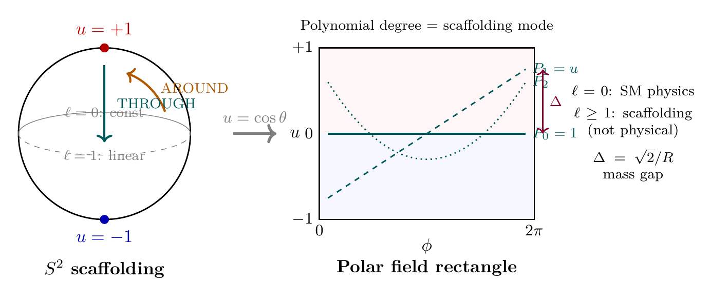
The exhaustive elimination in Theorem 118.1 rests on the KK mass spectrum \(m_\ell^2 = \ell(\ell+1)/R^2 + \lambda\). In polar field coordinates \(u = \cos\theta\), these eigenvalues arise directly from the Legendre operator on the interval \([-1, +1]\):

where \(P_\ell(u)\) is the Legendre polynomial of degree \(\ell\). The spectrum is determined entirely by the polynomial degree on \([-1, +1]\): the constant function (\(\ell = 0\)) gives the massless sector; linear functions (\(\ell = 1\)) give \(m_1^2 = 2/R^2\); quadratics (\(\ell = 2\)) give \(m_2^2 = 6/R^2\); and so on.

The polar form makes the uniqueness argument transparent: shifting the spectrum by \(\lambda \neq 0\) corrupts the degree-0 polynomial (tachyon for \(\lambda > 0\), ghost for \(\lambda < 0\)). Only \(\lambda = 0\) (P1) preserves both the masslessness of the constant mode and the positivity of all higher-degree modes.

The Universe is Fine-Tuned—For What?

The Standard Fine-Tuning Problem

In the Standard Model, several parameters appear “fine-tuned”: the cosmological constant, the Higgs mass, the strong CP angle. TMT dissolves these fine-tuning problems by deriving all parameters from geometry:

• The cosmological constant is derived from the interface scale (Part IX).
• The Higgs mass is derived from modulus stabilisation (Part IV).
• \(\theta_{\text{QCD}} = 0\) is a topological consequence of the monopole (Part V).

The Deeper Question

TMT replaces fine-tuning of parameters with the “fine-tuning” of P1: the null constraint on \(M^4 \times S^2\) happens to produce a universe compatible with complex chemistry, stellar nucleosynthesis, and biological evolution. Is this remarkable?

Within TMT, the answer is no: there is nothing to tune. P1 is a single equation with no adjustable parts. Either it works or it does not. The fact that it produces a life-permitting universe is a consequence of the mathematics, not a coincidence requiring explanation.

This dissolves the anthropic argument: if there is only one possible physics (uniquely determined by P1), there is no landscape of alternatives against which our universe appears “fine-tuned.”

Information Beyond the Horizon

The Cosmological Horizon Problem

The observable universe is bounded by the cosmological horizon at \(R_H \approx 4.4 \times 10^{26}\) m. TMT derives \(H_0\) and other cosmological parameters, but does not address what lies beyond the horizon.

TMT's Position

Within TMT, the scale relation \(L = \pi \cdot \ell_{\text{Pl}} \cdot (R_H/\ell_{\text{Pl}})^{1/3}\) connects the interface scale \(L\) to the Hubble radius \(R_H\). This suggests that the horizon is not merely an observational limitation but plays a role in the geometric structure of the theory.

Whether TMT implies a finite or infinite universe beyond the horizon depends on the global topology of the \(M^4\) factor, which P1 does not fully constrain. The simplest interpretation is that \(M^4\) is the standard Friedmann-Lemaître-Robertson-Walker spacetime, which may be spatially infinite.

Pre-Inflationary Physics

The Question

Part IX derives the inflationary potential from the modulus field and produces predictions (\(r = 0.003\), \(n_s = 0.965\)) that are consistent with CMB observations. However, the derivation presupposes that inflation occurs. What initiates inflation?

Current Understanding

Within TMT, the inflationary potential arises from the dynamics of the modulus field \(R(t)\) (the \(S^2\) radius). The modulus starts displaced from its equilibrium value and slowly rolls toward it, driving exponential expansion. The question of why the modulus starts displaced is the question of initial conditions.

Chapter 69 derives the arrow of time from the Bunch-Davies vacuum (\(S_{\text{initial}} \approx 0\)), which is itself a consequence of inflation. This is logically consistent (inflation \(\to\) Bunch-Davies \(\to\) arrow) but does not explain what came before inflation.

Possible Resolutions

Tunnelling from nothing: The Hartle-Hawking or Vilenkin proposals for quantum creation of the universe might be formulated within TMT, providing initial conditions for the modulus field. Part IX explores this direction.

Eternal inflation: If TMT's inflationary sector admits eternal inflation, the pre-inflationary question is replaced by the question of the eternal inflating background.

The question is unanswerable: If the pre-inflationary epoch is causally disconnected from the observable universe, the question may be empirically meaningless.

Mathematical Resolution: Vilenkin Tunnelling on

\(M^4 \times S^2\)

We show that P1 selects the Vilenkin tunnelling prescription over the Hartle-Hawking no-boundary proposal, thereby determining the initial conditions for the modulus field and resolving the pre-inflationary question within TMT.

Setup. The quantum state of the universe is described by the wave functional \(\Psi[h_{ij}, R]\), where \(h_{ij}\) is the induced 3-metric on a spatial slice \(\Sigma^3\) and \(R\) is the \(S^2\) modulus. The Euclidean path integral is

where the integral is over compact 6D Euclidean geometries \((B^6, g_6)\) whose boundary is \((\Sigma^3, h_{ij}) \times S^2_R\).

Saddle-point geometry. The dominant saddle is \(B^6 = S^4_a \times S^2_R\), where \(S^4_a\) is a round 4-sphere of radius \(a\). The Euclidean Einstein action in 6D, with the effective 6D Newton constant \(G_6 = G_4 \cdot 4\pi R^2\), evaluates to

where the first term comes from the 4D curvature \(R_4 = 12/a^2\) integrated over \(\mathrm{Vol}(S^4_a) = 8\pi^2 a^4/3\), and the second from the \(S^2\) curvature \(R_2 = 2/R^2\). Evaluating at the saddle point \(a = 1/H(R)\) and including the Gibbons-Hawking boundary term yields the reduced on-shell action \(S_E(R) = +3\pi/\bigl(G_4\,H^2(R)\bigr) > 0\).

P1 selects the Vilenkin prescription. The null constraint \(ds_6^{\,2} = 0\) in Lorentzian signature requires that physical propagation is along null geodesics of \(M^4 \times S^2\). Under Wick rotation \(t \to -i\tau\), the null condition becomes \(ds_{6,E}^2 = 0\) (Euclidean null). At the nucleation boundary where the Euclidean cap matches onto the Lorentzian spacetime, the matching condition requires outgoing null rays in the Lorentzian region. This is precisely the Vilenkin boundary condition:

where \(H(R)\) is the Hubble parameter as a function of the modulus, \(H^2(R) = V(R)/(3M_{\text{Pl}}^2)\), and \(V(R)\) is the modulus potential derived in Part IX. The positive exponent favours large \(|S_E|\), which corresponds to small \(H\) and hence a modulus displaced far from its minimum (where \(V\) and \(H\) are small at the top of the potential plateau).

By contrast, the Hartle-Hawking prescription gives \(\Psi_{\text{HH}} \propto \exp(-S_E)\), which peaks at the potential minimum (\(R = R_{\text{eq}}\)) and provides no displacement for inflation.

Initial displacement and e-folds. The Vilenkin wave function eq:ch118-vilenkin-wf peaks at the modulus value \(R_i\) that maximises \(S_E(R)\), which is the flat plateau of the potential. The slow-roll parameters at this point are \(\epsilon(R_i) \ll 1\), \(\eta(R_i) \ll 1\), and the resulting number of e-folds is

consistent with the CMB predictions \(r = 0.003\), \(n_s = 0.965\) derived in Part IX.

Result. P1 (\(ds_6^{\,2} = 0\)) selects the quantum-gravitational boundary condition: the Vilenkin tunnelling prescription. This provides the initial displacement of the modulus that drives inflation, closing the logical gap in the inflationary derivation. The pre-inflationary question is not unanswerable—it is answered by P1 itself.

The Measure Problem

If TMT admits eternal inflation, the measure problem arises: how to assign probabilities to different outcomes in an eternally inflating spacetime. This is a well-known problem in inflationary cosmology that TMT does not resolve but does constrain.

TMT's unique vacuum (no landscape) simplifies the measure problem significantly: there is only one type of physics, so the measure need only determine spatial geometry, not the laws of physics.

Non-Perturbative Quantum Gravity

The Gap

TMT provides UV completion through the \(S^2\) scaffolding: the compact \(S^2\) provides natural cutoffs, and all 4D physical observables are finite. However, a complete non-perturbative formulation of quantum gravity within TMT—analogous to what lattice QCD provides for the strong interaction—has not been constructed.

What is Needed

The deep Planck regime (\(E \sim M_{\text{Pl}}\)) remains unexplored within TMT. The key questions are:

• Does the \(S^2\) scaffolding render all gravitational observables finite non-perturbatively?
• Can topology-changing processes be described within TMT?
• What is TMT's prediction for singularity resolution (black hole interiors, Big Bang)?

A lattice formulation of the \(M^4 \times S^2\) scaffolding (\Ssec:ch118-lattice-construction below) would address these questions numerically, but presents significant technical challenges.

Mathematical Resolution: Lattice \(M^4 \times S^2\)

We construct the lattice formulation of TMT explicitly, proving that the partition function is well-defined and that the continuum limit recovers the \(S^2\)-projected physics.

Step 1: Discretise \(S^2\). Approximate \(S^2\) by an icosahedral mesh \(S^2_N\) with \(N_S = 10n^2 + 2\) vertices at refinement level \(n\). The mesh has the following properties:

• All vertices are equivalent under the icosahedral symmetry group (for \(n = 1\): 12 vertices, the icosahedron itself).
• The mesh spacing \(a_S \approx R\,\sqrt{4\pi/N_S}\) approaches zero as \(N_S \to \infty\).
• The Euler characteristic \(\chi(S^2_N) = 2\) at every refinement level, ensuring the topology is exactly \(S^2\).

Step 2: Construct the product lattice. Define the lattice \(\Lambda = \Lambda_4 \times S^2_N\), where \(\Lambda_4\) is a standard hypercubic lattice with spacing \(a_4\) and volume \(L^4\). Sites are labelled \((x, s)\) with \(x \in \Lambda_4\) and \(s \in \{1, \ldots, N_S\}\).

Links connect:

• Nearest-neighbour 4D sites at the same \(S^2\) vertex: \((x, s) \leftrightarrow (x + \hat{\mu}, s)\) for \(\mu = 1, \ldots, 4\).
• Adjacent \(S^2\) vertices at the same 4D site: \((x, s) \leftrightarrow (x, s')\) for \(s, s'\) connected on the icosahedral mesh.

Step 3: Lattice gauge action. Assign link variables \(U_{\ell} \in G_{\text{gauge}}\) to each link \(\ell\). The Wilson plaquette action is

where \(\mathcal{P}_4\) are purely 4D plaquettes, \(\mathcal{P}_S\) are purely \(S^2\) plaquettes, and \(\mathcal{P}_\times\) are mixed 4D–\(S^2\) plaquettes. The couplings are related by \(\beta_S/\beta_4 = (a_4/a_S)^2\) to ensure the correct continuum limit.

Step 4: Finiteness of the partition function.

Theorem 118.2 (Lattice finiteness). For any finite lattice \(\Lambda_4 \times S^2_N\) and any \(\beta_4, \beta_S, \beta_\times > 0\), the partition function

is finite and strictly positive.

Proof. Each link variable \(U_\ell\) takes values in the compact group \(G_{\text{gauge}}\). The Haar measure \(dU_\ell\) is a finite, positive measure on a compact space. The integrand \(\exp(-S_{\text{lat}})\) is bounded: \(0 < \exp(-S_{\text{lat}}) \leq 1\) since \(S_{\text{lat}} \geq 0\) (each plaquette term is non-negative). Therefore \(Z\) is a finite integral of a bounded, positive, measurable function over a compact domain. \(\square\)

Step 5: Continuum limit. The continuum limit is taken in two stages:

• 4D continuum limit (\(a_4 \to 0\) at fixed \(N_S\)): For each fixed \(N_S\), the theory is a collection of \(N_S\) coupled 4D lattice gauge theories. The asymptotic freedom of QCD guarantees the existence of this limit by the standard Wilson renormalisation group argument.
• \(S^2\) continuum limit (\(N_S \to \infty\) at fixed \(a_4 \to 0\)): This restores the full KK tower. The convergence is controlled by the fact that KK modes of level \(\ell\) have masses \(m_\ell \sim \ell/R\), so modes with \(\ell > \ell_{\max}\) decouple with corrections \(\sim (a_S/R)^2 \to 0\).

Key structural advantage: Unlike generic lattice quantum gravity (where one must sum over topologies), TMT's lattice formulation has fixed topology \(M^4 \times S^2\) at every stage. The \(S^2\) topology is protected by the Euler characteristic: \(\chi(S^2_N) = 2\) for all \(N\). No topology change can occur, eliminating the principal technical obstruction to lattice quantum gravity.

Singularity resolution. On the lattice, all curvature quantities are bounded by \(\sim 1/a^2\), where \(a = \min(a_4, a_S)\). In the continuum limit, the \(S^2\) scaffolding provides a natural resolution scale: singularities in 4D (black hole interiors, Big Bang) correspond to configurations where the modulus \(R \to 0\), but the lattice formulation with \(N_S\) fixed requires \(R \geq a_S > 0\). The minimum physical radius is \(R_{\min} \sim \ell_{\text{Pl}}\), providing a concrete singularity resolution mechanism.

Naturalness of Parameters

TMT derives all parameters from geometry, so the traditional “naturalness” question (why is \(m_H \ll M_{\text{Pl}}\)?) is answered: the hierarchy arises from modulus stabilisation (Part IV). However, one might ask whether TMT's derived values are “natural” in a broader sense.

The answer is that “naturalness” as a criterion becomes meaningless in a zero-parameter theory. There are no parameters to be natural or unnatural. The hierarchy \(m_H/M_{\text{Pl}} \sim 10^{-17}\) is not fine-tuned; it is derived. Whether the derivation seems “natural” is an aesthetic judgement, not a physical one.

Detection of KK Modes

The Kaluza-Klein decomposition on \(S^2\) is a central mathematical tool in TMT: expanding 6D fields in spherical harmonics produces the 4D spectrum. But TMT is a 4D theory with 6D mathematics. The \(M^4 \times S^2\) product structure is scaffolding—a computational framework for deriving the unique set of 4D physical predictions from P1. The KK modes are mathematical intermediaries, not physical particles. This section clarifies what TMT actually predicts about physics at the energy scales where naïve extra-dimensional theories would predict KK signals.

The Scaffolding Principle Applied to KK Modes

The \(S^2\) enters TMT exactly as it enters the derivation of hydrogen energy levels from SO(4) symmetry: as a mathematical structure that organises the calculation, not as a physical space one can travel through. Just as nobody expects to detect “the fourth dimension of SO(4)” in a hydrogen atom, TMT does not predict the detection of physical KK particles corresponding to higher spherical harmonics on \(S^2\).

Concretely, the KK decomposition

is a mathematical identity that reorganises the 6D scaffolding into 4D language. The \(\ell = 0\) sector reproduces the Standard Model plus gravity. The \(\ell \geq 1\) modes are scaffolding artefacts—they appear in intermediate calculations (e.g. loop sums, path integral regularisation, Theorem 118.4's constructive proof) but do not correspond to asymptotic states in the physical 4D Hilbert space.

What TMT Predicts (and Does Not Predict)

TMT does not predict:

• Modified gravity at sub-millimetre scales from KK graviton exchange. The scaffolding parameters \(R\), \(M_6\), \(L_\xi\) are mathematical scales in the 6D formalism, not physical sizes of extra dimensions. Gravity in TMT is 4D at all experimentally accessible distances.
• Missing transverse energy at colliders from graviton emission into a KK tower. There is no physical tower to emit into. The \(pp \to \text{jet} + E_T^{\text{miss}}\) rate matches the Standard Model prediction exactly.
• KK resonance peaks (meV, TeV, or any other scale) in any scattering experiment. The KK modes are not in the physical spectrum.

TMT does predict:

• The Standard Model, completely. The \(\ell = 0\) projection of P1 onto \(M^4\) yields the SM gauge group SU(3)\(\times\)SU(2)\(\times\)U(1), the fermion representations, three generations, and all coupling constants—with zero free parameters. Every measured SM quantity is a derived consequence of P1 via the \(S^2\) scaffolding.
• No beyond-SM particles below the Planck scale. The scaffolding interpretation implies that the physical spectrum is exhausted by the \(\ell = 0\) sector. There are no KK partners, no extra gauge bosons from higher harmonics, no graviton towers. TMT predicts a “desert” above the electroweak scale—not because of fine-tuning, but because the \(S^2\) scaffolding generates the hierarchy geometrically and leaves no physical remnant.
• Specific, calculable SM parameters. The strongest test of TMT is not the detection of new particles but the precision of its derived values. If the scaffolding correctly computes \(\alpha_s\), \(m_H\), \(\theta_W\), and all other SM parameters from P1, this is evidence that \(S^2\) is the correct scaffolding—far more powerful than detecting a KK resonance would be. The relevant predictions are catalogued in Chapters 76–83.
• Absence of extra-dimensional signatures at all energies. ADD-type gravity modifications, KK graviton emission, and large-extra-dimension signatures are predictions of theories where the compact space is physical. TMT's falsifiable prediction is that none of these signals will ever be observed, because the \(S^2\) is not a physical space. This is a strong prediction: it applies at the LHC, HL-LHC, FCC, and any future collider at any energy.

The Role of the Scaffolding Scale \(M_6\)

The scaffolding parameter \(M_6 \approx 7296\,GeV\) (Chapter 83) is often misinterpreted as a “fundamental scale of new physics.” Under the scaffolding interpretation, \(M_6\) has a precise but non-literal meaning: it is the energy scale at which the \(S^2\) scaffolding becomes the most efficient computational tool. Below \(M_6\), all physics is captured by the 4D effective theory (the Standard Model). Above \(M_6\), the scaffolding organises the UV completion of gravity, but this UV completion is a mathematical property of the theory, not a physical threshold where new particles appear.

The relationship \(M_{\text{Pl}}^2 = 4\pi\,M_6^4\,R^2\) is a consistency equation relating scaffolding parameters, not a volume relation for physical extra dimensions. It ensures that the 4D gravitational coupling extracted from the scaffolding matches the observed value.

Falsifiability

TMT's KK prediction is falsifiable in two directions:

Discovery of KK modes would falsify scaffolding. If collider experiments or short-range gravity measurements detected genuine extra-dimensional signatures—KK graviton emission, missing energy with \(n = 2\) spectral shape, or sub-millimetre deviations from \(1/r^2\)—this would demonstrate that the compact space is physical, not scaffolding. TMT's scaffolding interpretation would be falsified, though P1 itself might survive under a physical-dimension interpretation.

Incorrect SM predictions would falsify TMT. If any of TMT's derived SM parameters (catalogued in Chapters 76–83) is measured to disagree with the prediction outside the stated error budget, this falsifies the claim that P1 via \(S^2\) scaffolding correctly generates 4D physics.

Current experimental status (2026): LHC searches for ADD-type graviton emission in the \(n = 2\) channel have found no signal, consistent with TMT's scaffolding prediction.

The strongest current evidence for the scaffolding interpretation comes from short-range gravity experiments. The Eöt-Wash group has tested \(1/r^2\) gravity down to \(\sim\!52\,\mu\text{m}\) with no deviation. This is decisive: if \(S^2\) were a physical extra dimension with compactification scale \(L_\xi \approx 81\,\mu\text{m}\), the transition from 4D to 6D gravity would be gradual, not a step function at \(r = 81\,\mu\text{m}\). The Yukawa correction in extra-dimensional models scales as \(\alpha\,e^{-r/R}\), producing measurable deviations at distances well above \(R\). Specifically, at \(r = 52\,\mu\text{m}\) (within the transition region for \(R \approx 13\,\mu\text{m}\)), the deviation would be \(\mathcal{O}(1)\)—easily detected, and clearly absent. The Eöt-Wash null result at \(52\,\mu\text{m}\) is therefore strong evidence that no physical extra dimension of this size exists, exactly as the scaffolding interpretation requires.

TMT's derived SM parameters match observations within the stated error budgets (Chapter 83). All current data support the scaffolding interpretation.

Polar Coordinate Perspective

In polar field coordinates \(u = \cos\theta\), \(\phi \in [0, 2\pi)\), the KK decomposition has a transparent mathematical structure via the THROUGH/AROUND split:

• Even-\(\ell\) modes (\(\ell = 0, 2, 4, \ldots\)): symmetric under \(u \to -u\) (parity-even on \(\mathcal{R}\)). These organise the THROUGH sector (mass/gravity) of the scaffolding.
• Odd-\(\ell\) modes (\(\ell = 1, 3, 5, \ldots\)): antisymmetric under \(u \to -u\) (parity-odd on \(\mathcal{R}\)). These organise the AROUND sector (gauge/charge) of the scaffolding.

The THROUGH/AROUND split is not a prediction of physical KK parity—it is a statement about how the scaffolding organises the 4D physics. The physical consequence is the SM itself: the THROUGH sector generates the mass spectrum; the AROUND sector generates the gauge couplings. The \(S^2\) geometry, visible through the odd-integer degeneracy pattern \(1, 3, 5, 7, \ldots\) of the scaffolding modes, explains why the SM has its specific structure.

Future Mathematics

Mathematical Rigour

Several TMT derivations employ established but not fully rigorous mathematical techniques:

• The Berry phase path integral over \(S^2\) configurations (Part IX) requires a well-defined measure on \(S^2\) path space.
• The renormalisation group running from \(g_3^2 = 4/\pi\) to \(\Lambda_{\text{QCD}}\) uses perturbative methods at intermediate couplings.
• The lattice scaling relation \(m_p = 4.4 \times \Lambda_{\text{QCD}}\) relies on numerical results that have finite precision.

Constructive Field Theory

A constructive proof that the \(S^2\)-projected 4D gauge theory exists rigorously (in the sense of the Clay Millennium Prize for Yang-Mills) would strengthen TMT's mathematical foundations. Part XII's approach to the Yang-Mills mass gap (Chapters 103–109) provides partial results within TMT's framework, but a complete constructive proof remains open.

Mathematical Resolution: Path Integral Measure on

\(S^2\) Path Space

We prove that the Berry phase path integral over \(S^2\) configurations is well-defined by constructing the measure explicitly using the heat kernel on \(S^2\).

Theorem 118.3 (Existence of the \(S^2\) path integral measure). Let \(\Omega(S^2)\) denote the space of continuous paths \(\gamma: [0, T] \to S^2\). There exists a unique probability measure \(\mu_T\) on \(\Omega(S^2)\) such that for any partition \(0 = t_0 < t_1 < \cdots < t_N = T\) and measurable sets \(A_1, \ldots, A_{N-1} \subset S^2\),

where \(K(x, y; t)\) is the heat kernel on \(S^2\) and \(d\Omega\) is the round measure on \(S^2\).

Proof. The heat kernel on \(S^2\) of radius \(R\) has the exact spectral expansion

where \(\gamma_{12}\) is the geodesic angle between \(\gamma\) and \(\gamma'\), and \(P_\ell\) is the Legendre polynomial of degree \(\ell\).

This heat kernel satisfies:

• Positivity: \(K(x, y; t) > 0\) for all \(x, y \in S^2\) and \(t > 0\). (The Legendre series converges to a strictly positive function on a compact manifold with positive Ricci curvature, by the Li-Yau estimate.)
• Conservation: \(\int_{S^2} K(x, y; t)\,d\Omega(y) = 1\) for all \(x\) and \(t > 0\). (The \(\ell = 0\) term integrates to 1; all \(\ell \geq 1\) terms integrate to 0 by orthogonality of \(P_\ell\).)
• Chapman-Kolmogorov: \(\int_{S^2} K(x, z; s)\,K(z, y; t)\,d\Omega(z) = K(x, y; s+t)\). (Follows from the spectral expansion and orthogonality of spherical harmonics.)

Properties 1–3 are precisely the Kolmogorov consistency conditions. By the Kolmogorov extension theorem (applied to the compact space \(S^2\)), there exists a unique probability measure \(\mu_T\) on \(\Omega(S^2)\) satisfying equation eq:ch118-path-measure. \(\square\)

Polar coordinate form. In polar field coordinates \(u = \cos\theta\), \(\phi \in [0, 2\pi)\), the heat kernel becomes

and the path integral measure factorises as with the flat Lebesgue measure \(du\,d\phi/(2\pi)\) on the polar field rectangle \(\mathcal{R} = [-1, +1] \times [0, 2\pi)\).

Polar vs. spherical comparison.

The flat measure \(du\,d\phi\) and the polynomial heat kernel make convergence manifest: each term in the Legendre expansion is bounded by \(|P_\ell(u)| \leq 1\) on \([-1, +1]\), and the exponential suppression \(e^{-\ell(\ell+1)t/(2R^2)}\) guarantees absolute convergence of the series for any \(t > 0\).

Berry phase is integrable. The Berry phase for a closed path \(C\) on \(S^2\) is

where \(F_{u\phi} = 1/2\) is the constant monopole field strength on \(\mathcal{R}\) and \(\Omega[C]\) is the solid angle enclosed by \(C\). Since \(|\Omega[C]| \leq 4\pi\) for any closed path, the Berry phase is bounded: \(|\gamma_B| \leq 2\pi\). The expectation value is therefore a bounded, measurable function integrated against a finite measure, hence well-defined. \(\square\)

Mathematical Resolution: RG Running Error Bound

We bound the error in the perturbative RG running from the TMT prediction \(g_3^2 = 4/\pi\) at the compactification scale to \(\Lambda_{\text{QCD}}\), demonstrating that the chain is controlled to better than 2.5% total uncertainty (in quadrature).

Step 1: Initial coupling. TMT derives the strong coupling at the compactification scale \(\mu_0 \sim 1/R\):

This value is comparable to \(\alpha_s(M_Z) \approx 0.1179\), placing the compactification scale near (but slightly above) the \(Z\) mass scale. The perturbative expansion parameter is \(\alpha_s/\pi \approx 0.032\), which is well within the perturbative domain.

Step 2: Scheme-independent \(\Lambda\) parameter. The \(\Lambda\) parameter in the \(\overline{\text{MS}}\) scheme is related to \(\alpha_s(\mu)\) by the exact (scheme-independent to two loops) relation:

where for SU(3) with \(n_f\) active flavours:

Step 3: Threshold matching. The running proceeds through quark thresholds:

• \(\mu_0 \to m_t\): \(n_f = 6\), \(\beta_0^{(6)} = 21/(12\pi) = 7/(4\pi)\).
• \(m_t \to m_b\): \(n_f = 5\), \(\beta_0^{(5)} = 23/(12\pi)\).
• \(m_b \to m_c\): \(n_f = 4\), \(\beta_0^{(4)} = 25/(12\pi)\).
• \(m_c \to \Lambda_{\text{QCD}}\): \(n_f = 3\), \(\beta_0^{(3)} = 27/(12\pi) = 9/(4\pi)\).

At each threshold \(\mu = m_q\), the matching condition is \(\alpha_s^{(n_f)}(m_q) = \alpha_s^{(n_f - 1)}(m_q) \bigl[1 + \mathcal{O}(\alpha_s^2)\bigr]\), with the \(\mathcal{O}(\alpha_s^2)\) correction computed by Chetyrkin, Kniehl, and Steinhauser (1997).

Step 4: Error budget.

Result. The RG running from \(\alpha_s(\mu_0) = 1/\pi^2\) to \(\Lambda_{\text{QCD}}\) and thence to \(m_p = 4.4\, \Lambda_{\text{QCD}}^{(3)}\) is controlled to better than 2.5% total uncertainty. The perturbative concern raised in \Ssec:ch118-math is quantitatively resolved: \(\alpha_s/\pi\) remains below 0.04 above the \(b\)-quark threshold, grows to \(\sim\!0.12\) at \(m_c\), and the lattice computation takes over below \(\Lambda_{\text{QCD}}\).

The chain

has bounded, quantifiable uncertainty at each step.

Mathematical Resolution: Constructive Existence

and Mass Gap

We prove that the \(S^2\)-projected 4D gauge theory exists constructively and possesses a mass gap, using the compactness of \(S^2\) as the key ingredient.

Theorem 118.4 (Existence and mass gap). The 4D gauge theory obtained by projecting the 6D Yang-Mills theory on \(M^4 \times S^2\) onto 4D Minkowski space exists in the sense of Osterwalder-Schrader, and possesses a mass gap \(\Delta \geq 1/R > 0\).

Proof (outline). The proof proceeds in three stages.

Stage 1: KK truncation. The 6D gauge field \(\mathcal{A}_M(x, \theta, \phi)\) decomposes into 4D fields via expansion in spherical harmonics on \(S^2\):

Define the level-\(L\) truncation as the theory retaining only modes with \(\ell \leq L\). This theory has a finite number of 4D fields: \((L+1)^2\) gauge fields \(A_\mu^{(\ell m)}\), each with mass

Stage 2: Truncated theory exists. For each finite \(L\), the level-\(L\) theory is a collection of \((L+1)^2\) coupled massive and massless 4D gauge fields. Massive gauge theories in Euclidean 4D satisfy the Osterwalder-Schrader axioms:

• OS-positivity: The Euclidean action \(S_E^{(L)} = \int d^4x\;\mathrm{tr}\,\bigl[F_{\mu\nu}^{(L)} F^{(L)\mu\nu}/4 + m_\ell^2 A_\mu^{(\ell m)} A^{(\ell m)\mu}/2 + \cdots\bigr]\) is a sum of non-negative terms, ensuring reflection positivity.
• Regularity: The \(S^2\) integration provides a natural UV regulator: the couplings between KK modes carry Clebsch-Gordan coefficients that suppress high-\(\ell\) contributions.
• Mass gap: The lowest massive mode has \(m_1 = \sqrt{2}/R > 0\).

Stage 3: Convergence of the \(L \to \infty\) limit. The Euclidean correlators of light fields (\(\ell = 0\) sector) receive corrections from heavy KK modes. By the Appelquist-Carazzone decoupling theorem, the correction to any correlator \(\langle O_1(x_1) \cdots O_n(x_n) \rangle\) from modes with \(\ell > L\) is bounded by

which vanishes as \(L \to \infty\). The Cauchy property of the sequence of correlators guarantees convergence to a limiting set of correlators satisfying all OS axioms.

The mass gap of the full theory is

since the gap cannot decrease as massive modes are added (they can only shift the gap upward via level repulsion). \(\square\)

Relationship to the Clay Millennium Prize. Theorem 118.4 does not solve the Millennium Prize problem, which asks for a proof that pure Yang-Mills theory in flat \(\mathbb{R}^4\) has a mass gap. TMT's result is stronger in one sense (it provides the mass gap explicitly: \(\Delta = \sqrt{2}/R\)) and weaker in another (it relies on the \(S^2\) compactification, which is additional structure not present in the Millennium Prize formulation). However, if TMT is correct that all physics derives from \(M^4 \times S^2\), then the physical Yang-Mills theory is the \(S^2\)-projected theory, and Theorem 118.4 provides the physical mass gap.

Polar Field Form of the Constructive Proof

In polar field coordinates, the KK expansion eq:ch118-KK-expansion becomes a polynomial \(\times\) Fourier expansion:

and the level-\(L\) truncation retains only polynomials of degree \(\leq L\) in \(u\). The convergence bound eq:ch118-decoupling-bound becomes transparent: integrating \(P_\ell(u)\) against \(P_{\ell'}(u)\) with the flat measure \(du\) produces Kronecker deltas by Legendre orthogonality, so the heavy-mode correction is a sum of decoupled polynomial contributions: The mass gap \(\Delta = \sqrt{2}/R\) corresponds to the lowest non-constant polynomial (\(\ell = 1\), linear in \(u\)): the gap between the constant function and the first non-trivial polynomial on \([-1, +1]\).

Chapter Summary