Chapter 64

Classical Dynamics on S²

Introduction

The previous chapters have derived the TMT cosmological framework (Chapter 57) and the gravitational sector (Chapters 51–56) from the single postulate P1: $ds_6^{\,2}=0$. Before turning to inflation (Chapter 59), we must establish the classical dynamical framework on the $S^2$ scaffolding, because inflation in TMT is a process by which the $S^2$ structure transitions from a quantum to a classical regime.

This chapter develops two essential mathematical structures: the phase space on the compact manifold $S^2$ (Section sec:ch58-phase-space), and the momentum maps and conservation laws that arise from the $SO(3)$ isometry group (Section sec:ch58-momentum-maps). These structures underpin the inflationary dynamics of the modulus field and the emergence of gauge symmetries from geometry.

Scaffolding Interpretation

The $S^2$ is mathematical scaffolding (Part A). “Classical dynamics on $S^2$” refers to the mathematical structure of the mode decomposition and its classical limit, not to literal particle motion in extra dimensions. The physical consequence is the structure of the 4D effective field theory that governs inflation and gauge interactions.

Phase Space on the Compact Manifold

The Round $S^2$ as a Symplectic Manifold

The round 2-sphere of radius $R_0$ has the metric:

$$ ds_{S^2}^2 = R_0^2\,(d\theta^2 + \sin^2\theta\,d\phi^2) $$ (64.1)

with $\theta\in[0,\pi]$, $\phi\in[0,2\pi)$.

The $S^2$ carries a natural symplectic structure given by the area form (volume form on $S^2$):

$$ \omega = R_0^2\,\sin\theta\,d\theta\wedge d\phi $$ (64.2)

This 2-form is closed ($d\omega=0$, since $\omega$ is a top form on the 2-manifold) and nondegenerate (it vanishes nowhere on $S^2$). Therefore $(S^2,\omega)$ is a symplectic manifold.

Theorem 64.1 ($S^2$ as Symplectic Manifold)

The round 2-sphere $(S^2,\omega)$ with the area form $\omega=R_0^2\sin\theta\,d\theta\wedge d\phi$ is a compact symplectic manifold. The total symplectic volume is:

$$ \int_{S^2}\omega = 4\pi R_0^2 $$ (64.3)

Proof.

Step 1: Closedness: $d\omega=0$ because $\omega$ is a 2-form on a 2-dimensional manifold (all 3-forms on $S^2$ vanish).

Step 2: Nondegeneracy: In coordinates $(\theta,\phi)$, the matrix representation of $\omega$ is:

$$\begin{aligned} \omega_{ij} = R_0^2\sin\theta \begin{pmatrix} 0 & 1 \\ -1 & 0 \end{pmatrix} \end{aligned}$$ (64.4)

This has determinant $R_0^4\sin^2\theta>0$ for $\theta\in(0,\pi)$. At the poles $\theta=0,\pi$, the coordinate system degenerates but the form is smooth (as can be verified in stereographic coordinates).

Step 3: Total volume:

$$ \int_{S^2}\omega = R_0^2\int_0^{2\pi}d\phi\int_0^\pi\sin\theta\,d\theta = R_0^2\cdot 2\pi\cdot 2 = 4\pi R_0^2 $$ (64.5)

(See: Standard differential geometry; Part 3 \S7.1) □

Polar Field Form of the Symplectic Structure

The symplectic structure on $S^2$ takes its most transparent form in the polar field variable $u = \cos\theta$. Since $du = -\sin\theta\,d\theta$, the symplectic form (Eq. eq:ch58-symplectic-form) becomes:

$$ \omega = R_0^2\sin\theta\,d\theta \wedge d\phi = -R_0^2\,du \wedge d\phi $$ (64.6)

This is the standard Darboux form with constant coefficients. The $\sin\theta$ factor in the spherical expression was entirely a coordinate artifact—the symplectic structure on $S^2$ is intrinsically flat in the polar variable. The total symplectic volume becomes an elementary rectangle integral:

$$ \int_{S^2}\omega = R_0^2 \int_0^{2\pi} d\phi \int_{-1}^{+1} du = R_0^2 \times 2\pi \times 2 = 4\pi R_0^2 $$ (64.7)

The Poisson bracket on $S^2$ becomes the standard canonical form in the polar variable:

$$ \{f,g\}_{S^2} = \frac{1}{R_0^2}\left( \frac{\partial f}{\partial u}\frac{\partial g}{\partial\phi} - \frac{\partial f}{\partial\phi}\frac{\partial g}{\partial u} \right) $$ (64.8)

with the fundamental bracket:

$$ \{u,\phi\}_{S^2} = \frac{1}{R_0^2} $$ (64.9)

The polar variable $u$ and the azimuthal angle $\phi$ are canonically conjugate on $S^2$: the phase space of the 2-sphere IS the polar rectangle $[-1,+1]\times[0,2\pi)$ with constant symplectic area element $du\,d\phi$.

Property	Spherical $(\theta, \phi)$	Polar $(u, \phi)$
Symplectic form	$R_0^2\sin\theta\,d\theta\wedge d\phi$	$-R_0^2\,du\wedge d\phi$
Coefficient	$R_0^2\sin\theta$ (variable)	$R_0^2$ (constant)
Area element	$\sin\theta\,d\theta\,d\phi$ (curved)	$du\,d\phi$ (flat)
Position variable	$\phi \in [0,2\pi)$	$\phi \in [0,2\pi)$
Momentum variable	$\cos\theta$ (implicit)	$u$ (explicit)
Canonical bracket	$\\cos\theta,\phi\ = 1/R_0^2$	$\{u,\phi\} = 1/R_0^2$
Total volume	$\int\sin\theta\,d\theta\,d\phi$	$\int du\,d\phi = 4\pi$

The polar field variable $u = \cos\theta$ is not merely a convenient substitution—it is the natural canonical momentum on $S^2$. The Darboux theorem guarantees that every symplectic manifold admits local canonical coordinates; the polar variable provides a global Darboux chart on $S^2$ minus the poles, with the symplectic form having constant coefficients everywhere on the interior.

Scaffolding Interpretation

Scaffolding note: The polar field variable $u = \cos\theta$ is a coordinate choice, not a new physical assumption. The fact that $(S^2, \omega)$ becomes a flat rectangle $[-1,+1]\times[0,2\pi)$ in these coordinates verifies that the symplectic structure is the same—the $\sin\theta$ factor in the spherical representation was a coordinate artifact. All physical results (conservation laws, mode spectra, quantization) are identical in both coordinate systems.

Phase Space Coordinates

The symplectic structure on $S^2$ defines canonical coordinates. Using the Darboux-like coordinates $(q,p)=(\phi,\cos\theta)$, the symplectic form becomes:

$$ \omega = R_0^2\,dp\wedge dq = R_0^2\,d(\cos\theta)\wedge d\phi $$ (64.10)

In these coordinates:

$q=\phi\in[0,2\pi)$ plays the role of a “position” (azimuthal angle)
$p=\cos\theta\in[-1,1]$ plays the role of the conjugate “momentum” (related to the $z$-component of angular momentum)

Note that $p = \cos\theta = u$: the Darboux momentum IS the polar field variable. The “natural” phase space coordinates on $S^2$ discovered by the Darboux construction are precisely the polar coordinates $(u, \phi)$.

The Poisson bracket on $S^2$ is:

$$ \{f,g\}_{S^2} = \frac{1}{R_0^2\sin\theta}\left( \frac{\partial f}{\partial\theta}\frac{\partial g}{\partial\phi} - \frac{\partial f}{\partial\phi}\frac{\partial g}{\partial\theta} \right) $$ (64.11)

which in the polar variable takes the standard canonical form (Eq. eq:ch58-poisson-polar).

The Classical Hamiltonian on $S^2$

For a scalar field $\Phi$ on $M^4\times S^2$, the $S^2$ dynamics are governed by the Laplacian on the sphere. The classical Hamiltonian for the $S^2$ sector is:

$$ \mathcal{H}_{S^2} = \frac{1}{2R_0^2}\left[ \frac{1}{\sin\theta}\frac{\partial}{\partial\theta} \left(\sin\theta\frac{\partial}{\partial\theta}\right) + \frac{1}{\sin^2\theta}\frac{\partial^2}{\partial\phi^2} \right] = -\frac{\Delta_{S^2}}{2R_0^2} $$ (64.12)

where $\Delta_{S^2}$ is the Laplace–Beltrami operator on $S^2$.

Mode Decomposition and Energy Spectrum

The eigenfunctions of $\mathcal{H}_{S^2}$ are the spherical harmonics $Y_{lm}(\theta,\phi)$:

$$ -\Delta_{S^2}\,Y_{lm} = l(l+1)\,Y_{lm} $$ (64.13)

with eigenvalues $l(l+1)$, $l=0,1,2,\ldots$, and degeneracy $(2l+1)$ for each $l$.

The corresponding energy spectrum on $S^2$ is:

$$ E_l = \frac{l(l+1)}{2R_0^2} $$ (64.14)

Theorem 64.2 (Classical Mode Spectrum on $S^2$)

The classical dynamics on $S^2$ produce a discrete energy spectrum $E_l=l(l+1)/(2R_0^2)$ with the following mode classification relevant to TMT:

$l$	Modes	Energy	Physical Role
0	1	0	Modulus (size of $S^2$)
1	3	$1/R_0^2$	Gauge modes (absorbed into $SU(2)$)
$2$–$11$	140	$3/R_0^2$ to $66/R_0^2$	Stiffness modes
$\geq 12$	—	$\geq 78/R_0^2$	Truncated by topological cutoff

The topological cutoff $l_{\max}=D\chi-1=11$ ensures a finite number of physical modes.

Proof.

Step 1: The eigenvalue equation $-\Delta_{S^2}Y_{lm}=l(l+1)Y_{lm}$ is the standard result for the Laplacian on $S^2$ (ESTABLISHED).

Step 2: The mode classification follows from the physical role of each $l$-level in the TMT framework:

$l=0$: The single mode represents the overall size of $S^2$, i.e., the modulus field $\Phi$.
$l=1$: The three modes correspond to the three Killing vectors of $S^2$ and are absorbed into the $SU(2)$ gauge structure (Part 3, Theorem 7.5; Part 5 \S22.2).
$l=2$ to $l=11$: Shape deformation modes that contribute to gravitational stiffness (Part 5 \S22).

Step 3: The topological cutoff $l_{\max}=D\chi-1$ is derived in Part 5 \S22.3 from the requirement that the total mode count equals $(D\times\chi)^2=144$, giving $l_{\max}=11$ for $D=6$, $\chi(S^2)=2$.

Step 4: The mode sum for $l=2$ to $l=11$: $\sum_{l=2}^{11}(2l+1)=140$. These are the stiffness modes that generate the cosmic hierarchy $M_{\mathrm{Pl}}/H=e^{140.21}$ (Chapter 57).

(See: Part 3 \S7, Part 5 \S22) □

Polar Mode Decomposition: Polynomial $\times$ Fourier

In the polar field variable $u = \cos\theta$, the spherical harmonics decompose as:

$$ Y_{lm}(\theta,\phi) \;\longrightarrow\; N_{lm}\,P_l^{|m|}(u)\,e^{im\phi} $$ (64.15)

where $P_l^{|m|}(u)$ is the associated Legendre polynomial in $u$ and $N_{lm}$ is the normalization constant. This factorization is the THROUGH $\times$ AROUND decomposition made explicit:

THROUGH factor: $P_l^{|m|}(u)$ — a polynomial of degree $l$ in the polar variable $u \in [-1,+1]$. This carries the mass/gravitational physics (radial $S^2$ structure).
AROUND factor: $e^{im\phi}$ — a Fourier mode with winding number $m \in \{-l,\ldots,+l\}$. This carries the gauge/charge physics (azimuthal winding).

Orthogonality follows from the flat measure $du\,d\phi$:

$$ \int_{-1}^{+1}\!\!du \int_0^{2\pi}\!\!d\phi\; \overline{Y_{lm}}\,Y_{l'm'} = \delta_{ll'}\,\delta_{mm'} $$ (64.16)

where the THROUGH integral ($\int du$) and AROUND integral ($\int d\phi$) are independently evaluated as polynomial and Fourier orthogonality, respectively.

The mode classification from Theorem thm:P10-Ch58-spectrum acquires a transparent polar interpretation:

$l$	THROUGH (polynomial)	AROUND (Fourier)	Physical Role
0	$P_0(u) = 1$ (constant)	$m = 0$ only	Modulus (uniform on rectangle)
1	$P_1(u) = u$ (linear)	$m = 0, \pm 1$	Gauge ($u$-gradient + winding)
$2$–$11$	$P_l(u)$ (degree $l$)	$\|m\| \leq l$	Stiffness (polynomial $\times$ Fourier)

The Laplacian eigenvalue equation becomes the Legendre equation in $u$:

$$ \frac{d}{du}\!\left[(1-u^2)\frac{dP_l^m}{du}\right] + \left[l(l+1) - \frac{m^2}{1-u^2}\right]P_l^m = 0 $$ (64.17)

which is a polynomial eigenvalue problem on the flat domain $[-1,+1]$ — no trigonometric functions appear.

Phase Space Volume and Quantization

The symplectic structure on $S^2$ connects to the quantization of angular momentum. The total phase space volume is:

$$ \mathrm{Vol}(S^2) = \int_{S^2}\omega = 4\pi R_0^2 $$ (64.18)

By the Bohr–Sommerfeld quantization condition, the number of quantum states in a phase space region of volume $V$ is $V/(2\pi\hbar)$ (for each degree of freedom). For $S^2$:

$$ N_{\mathrm{states}} = \frac{4\pi R_0^2}{2\pi\hbar/p_0} = \frac{2R_0^2 p_0}{\hbar} $$ (64.19)

where $p_0$ is the characteristic momentum scale on $S^2$.

In TMT, with $R_0=L_\xi\approx81\,\mu\text{m}$, the mode spectrum is extremely dense at macroscopic scales but is truncated at $l_{\max}=11$ by the topological cutoff, giving a total of $(l_{\max}+1)^2=144$ modes.

Momentum Maps and Conservation

The $SO(3)$ Action on $S^2$

The isometry group of the round $S^2$ is $\mathrm{Iso}(S^2) =O(3)$, with connected component $SO(3)$ (Part 3, Theorem 7.1). The action of $SO(3)$ on $S^2$ is by rotations: each element $R\in SO(3)$ acts as a diffeomorphism $R:S^2\to S^2$ that preserves the metric and the symplectic form.

Theorem 64.3 ($SO(3)$ Symplectomorphism)

Every isometry of $(S^2,g)$ is a symplectomorphism of $(S^2,\omega)$:

$$ R^*\omega = \omega \quad\text{for all } R\in SO(3) $$ (64.20)

Proof.

Step 1: The symplectic form $\omega=R_0^2\sin\theta\, d\theta\wedge d\phi$ is the area form induced by the metric $g$.

Step 2: An isometry preserves the metric: $R^*g=g$.

Step 3: The area form is determined by the metric (it is the Riemannian volume form on a 2-manifold): $\omega=\sqrt{\det(g_{ij})}\,d\theta\wedge d\phi$.

Step 4: Since $R^*g=g$, the pullback preserves $\sqrt{\det(g_{ij})}$, and therefore $R^*\omega=\omega$.

(See: Part 3 \S7.1–7.2) □

Killing Vectors as Hamiltonian Vector Fields

The three Killing vector fields on $S^2$ (Part 3, Theorem 7.2):

$$\begin{aligned} \xi_1 &= -\sin\phi\,\partial_\theta - \cot\theta\cos\phi\,\partial_\phi \\ \xi_2 &= \cos\phi\,\partial_\theta - \cot\theta\sin\phi\,\partial_\phi \\ \xi_3 &= \partial_\phi \end{aligned}$$ (64.27)

satisfy the $\mathfrak{so}(3)$ Lie algebra: $[\xi_a,\xi_b]=\epsilon_{abc}\,\xi_c$.

Each Killing vector field is a Hamiltonian vector field with respect to the symplectic form $\omega$.

Theorem 64.4 (Momentum Map for $SO(3)$ on $S^2$)

The $SO(3)$ action on $(S^2,\omega)$ admits a momentum map $\mu:S^2\to\mathfrak{so}(3)^*\cong\mathbb{R}^3$ given by:

$$ \mu(\theta,\phi) = R_0^2\, \begin{pmatrix} \sin\theta\cos\phi \\ \sin\theta\sin\phi \\ \cos\theta \end{pmatrix} $$ (64.21)

The components $\mu_a=\iota_{\xi_a}\omega$ (the contraction of $\omega$ with the Killing vector $\xi_a$) are the Hamiltonian functions generating the $SO(3)$ action:

$$\begin{aligned} J_1 &= R_0^2\sin\theta\cos\phi \\ J_2 &= R_0^2\sin\theta\sin\phi \\ J_3 &= R_0^2\cos\theta \end{aligned}$$ (64.28)

These satisfy the Poisson bracket algebra:

$$ \{J_a,J_b\}_{S^2} = \epsilon_{abc}\,J_c $$ (64.22)

Proof.

Step 1: For $\xi_3=\partial_\phi$, compute the contraction $\iota_{\xi_3}\omega$:

$$\begin{aligned} \iota_{\partial_\phi}(R_0^2\sin\theta\,d\theta\wedge d\phi) &= R_0^2\sin\theta\, [d\theta(\partial_\phi)\,d\phi - d\phi(\partial_\phi)\,d\theta] \\ &= R_0^2\sin\theta\,[0\cdot d\phi - 1\cdot d\theta] \\ &= -R_0^2\sin\theta\,d\theta = d(R_0^2\cos\theta) \end{aligned}$$ (64.29)

Therefore $J_3=R_0^2\cos\theta$ generates rotations about the $z$-axis.

Step 2: For $\xi_1=-\sin\phi\,\partial_\theta -\cot\theta\cos\phi\,\partial_\phi$:

$$\begin{aligned} \iota_{\xi_1}\omega &= R_0^2\sin\theta\, [d\theta(\xi_1)\,d\phi - d\phi(\xi_1)\,d\theta] \\ &= R_0^2\sin\theta\, [(-\sin\phi)\,d\phi - (-\cot\theta\cos\phi)\,d\theta] \\ &= R_0^2[-\sin\theta\sin\phi\,d\phi + \cos\theta\cos\phi\,d\theta] \\ &= d(R_0^2\sin\theta\cos\phi) \end{aligned}$$ (64.30)

Therefore $J_1=R_0^2\sin\theta\cos\phi$.

Step 3: By an identical calculation (or by using the rotation $\phi\to\phi+\pi/2$): $J_2=R_0^2\sin\theta\sin\phi$.

Step 4: The Poisson brackets follow from the definition (Eq. eq:ch58-poisson):

$$\begin{aligned} \{J_1,J_2\}_{S^2} &= \frac{1}{R_0^2\sin\theta}\left( \frac{\partial J_1}{\partial\theta} \frac{\partial J_2}{\partial\phi} - \frac{\partial J_1}{\partial\phi} \frac{\partial J_2}{\partial\theta} \right) \\ &= \frac{1}{R_0^2\sin\theta}\left( R_0^2\cos\theta\cos\phi\cdot R_0^2\sin\theta\cos\phi - (-R_0^2\sin\theta\sin\phi)\cdot R_0^2\cos\theta\sin\phi \right) \\ &= \frac{R_0^2\cos\theta}{\sin\theta} (\sin\theta\cos^2\phi+\sin\theta\sin^2\phi) \\ &= R_0^2\cos\theta = J_3 \end{aligned}$$ (64.31)

Similarly, $\{J_2,J_3\}=J_1$ and $\{J_3,J_1\}=J_2$.

Step 5: The momentum map $\mu=R_0^2(\sin\theta\cos\phi,\sin\theta\sin\phi,\cos\theta)$ is equivariant: $\mu\circ R = \mathrm{Ad}^*_R\circ\mu$ for all $R\in SO(3)$, where $\mathrm{Ad}^*$ is the coadjoint action. This is verified by noting that $\mu$ is simply $R_0^2$ times the embedding $S^2\hookrightarrow\mathbb{R}^3$, and $SO(3)$ acts on $\mathbb{R}^3$ by the standard representation.

(See: Part 3 \S7.2, standard symplectic geometry) □

Polar Field Form of the Momentum Map

The momentum map acquires its most revealing form in the polar field variable $u = \cos\theta$. The three angular momentum components (Eqs. eq:ch58-J1–eq:ch58-J3) become:

$$\begin{aligned} J_3 &= R_0^2\,u \\ J_1 + iJ_2 &= R_0^2\,\sqrt{1-u^2}\;e^{i\phi} \end{aligned}$$ (64.32)

This is the crown jewel of the polar reformulation for this chapter: the $z$-component of angular momentum $J_3$ is linear in the polar variable—it IS the coordinate $u$ (up to the scale $R_0^2$). The Darboux canonical momentum $p = u$ and the angular momentum $J_3$ are the same quantity:

$$ J_3 = R_0^2\,u = R_0^2\,p $$ (64.23)

Meanwhile, $J_1 + iJ_2$ factorizes into THROUGH $\times$ AROUND: the modulus $\sqrt{1-u^2}$ depends only on $u$ (THROUGH direction, maximum at the equator $u = 0$, vanishing at the poles $u = \pm 1$), while the phase $e^{i\phi}$ depends only on $\phi$ (AROUND direction, winding number $+1$).

Component	Spherical	Polar	Character	Physical Role
$J_3$	$R_0^2\cos\theta$	$R_0^2 u$ (linear)	Pure THROUGH	Unbroken $U(1)_{\mathrm{em}}$
$J_1$	$R_0^2\sin\theta\cos\phi$	$R_0^2\sqrt{1{-}u^2}\cos\phi$	Mixed T$\times$A	Broken $W^\pm$ (real)
$J_2$	$R_0^2\sin\theta\sin\phi$	$R_0^2\sqrt{1{-}u^2}\sin\phi$	Mixed T$\times$A	Broken $W^\pm$ (imag)
$\|\mathbf{J}\|^2$	$R_0^4$	$R_0^4$	Casimir	Conserved magnitude

The Poisson algebra (Eq. eq:ch58-poisson-algebra) is verified directly from the canonical bracket $\{u,\phi\} = 1/R_0^2$:

$$ \{J_3, J_1+iJ_2\} = R_0^2\left\{u,\;\sqrt{1-u^2}\,e^{i\phi}\right\} = R_0^2 \cdot \frac{1}{R_0^2}\cdot i\sqrt{1-u^2}\,e^{i\phi} = i(J_1+iJ_2) $$ (64.24)

recovering the standard $\mathfrak{so}(3)$ ladder relation in one line, with no trigonometric identities required.

The polar reformulation makes the gauge structure geometrically literal:

$J_3$ conservation: The THROUGH coordinate $u$ is conserved under $\phi$-rotations — this is trivially evident from $\{u, \mathcal{H}\} = 0$ for any $\phi$-independent Hamiltonian. In 4D, this becomes conservation of the unbroken $U(1)_{\mathrm{em}}$ charge.
$J_1, J_2$ mix THROUGH and AROUND: The broken generators couple $u$-position to $\phi$-winding. Electroweak mixing IS around-through mixing on the polar rectangle (Chapter 15, \Ssec:ch58-polar-momentum-map).

Conservation Laws from Isometries

The momentum map provides the conservation laws on $S^2$.

Theorem 64.5 (Noether's Theorem on $S^2$)

For any $SO(3)$-invariant Hamiltonian $\mathcal{H}$ on $S^2$, the three angular momentum components $J_1,J_2,J_3$ are conserved:

$$ \frac{dJ_a}{dt} = \{J_a,\mathcal{H}\}_{S^2} = 0 \quad\text{for } a=1,2,3 $$ (64.25)

Moreover, the total angular momentum magnitude $|\mathbf{J}|^2=J_1^2+J_2^2+J_3^2=R_0^4$ is automatically conserved (it is a Casimir of the Poisson algebra).

Proof.

Step 1: By the definition of the Poisson bracket, if $\mathcal{H}$ is $SO(3)$-invariant, then $\mathcal{L}_{\xi_a} \mathcal{H}=0$ for each Killing vector $\xi_a$.

Step 2: Since $\xi_a$ is the Hamiltonian vector field of $J_a$, we have $\mathcal{L}_{\xi_a}\mathcal{H} =\{J_a,\mathcal{H}\}$.

Step 3: Therefore $\{J_a,\mathcal{H}\}=0$, and $J_a$ is conserved along the Hamiltonian flow.

Step 4: The Casimir property: $J_1^2+J_2^2+J_3^2=R_0^4(\sin^2\theta\cos^2\phi +\sin^2\theta\sin^2\phi+\cos^2\theta)=R_0^4$ is constant on $S^2$, hence trivially conserved.

(See: Noether's theorem, standard symplectic geometry) □

Physical Significance for TMT

The classical dynamics on $S^2$ have direct physical consequences in the TMT framework:

(1) Gauge symmetry from conservation: The three conserved angular momentum components $J_1,J_2,J_3$ on $S^2$ become the three generators of the $SU(2)$ gauge symmetry in 4D. The Killing vectors $\xi_a$ on $S^2$ become gauge fields $A_\mu^a(x)$ through the Kaluza–Klein mechanism (Part 3, Theorem 7.6):

$$ g_{\mu m}(x,\xi) = A_\mu^a(x)\,\xi_a^m(\xi) $$ (64.26)

Conservation of angular momentum on $S^2$ is equivalent to gauge invariance in 4D.

(2) Mode structure determines physics: The discrete energy spectrum $E_l=l(l+1)/(2R_0^2)$ determines which modes are physical:

The $l=0$ mode governs the modulus dynamics (inflation, dark energy)
The $l=1$ modes become gauge bosons
The $l\geq 2$ modes generate the cosmic hierarchy

(3) Phase space volume constrains quantization: The finite phase space volume $4\pi R_0^2$ of $S^2$, combined with the topological cutoff $l_{\max}=11$, gives exactly 144 quantum states. This is the origin of the $(D\chi)^2=144$ formula that determines the cosmic hierarchy (Part 5 \S22.3).

Table 64.1: Classical $S^2$ dynamics $\to$ 4D physics

$S^2$ Structure	4D Physics	Source
Isometry $SO(3)$	$SU(2)$ gauge symmetry	Part 3 \S7
Killing vectors $\xi_a$	Gauge fields $A_\mu^a$	Part 3 \S7.4
Momentum map $J_a$	Conserved charges	This chapter
Mode spectrum $E_l$	Particle/stiffness modes	Part 5 \S22
Symplectic volume $4\pi R_0^2$	$(D\chi)^2=144$ states	Part 5 \S22.3

**Figure 64.1:** Phase space of $S^2$ in polar field coordinates. **Left:** The $S^2$ sphere with angular momentum $J_3 = R_0^2\cos\theta$ along the THROUGH direction and azimuthal angle $\phi$ along the AROUND direction. The symplectic form has the variable coefficient $\sin\theta$. **Right:** In the polar variable $u = \cos\theta$, the phase space becomes the flat rectangle $[-1,+1]\times[0,2\pi)$ with *constant* symplectic form $\omega = -R_0^2\,du\wedge d\phi$. The canonical momentum IS $u$, and $J_3 = R_0^2 u$ is linear in the coordinate. Mode decomposition is polynomial (THROUGH) $\times$ Fourier (AROUND) on this flat domain.

Chapter Summary

Key Result

Classical Dynamics on $S^2$

The round 2-sphere $(S^2,\omega)$ is a compact symplectic manifold with the area form as its symplectic structure. The $SO(3)$ isometry group acts as symplectomorphisms, with the momentum map $\mu:S^2\to\mathbb{R}^3$ providing three conserved angular momentum components $J_a=R_0^2\hat{x}_a$ that satisfy $\{J_a,J_b\}=\epsilon_{abc}J_c$. The mode spectrum $E_l=l(l+1)/(2R_0^2)$ classifies fields into the modulus ($l=0$), gauge ($l=1$), and stiffness ($l\geq 2$) sectors. These structures directly determine the 4D physics: gauge symmetry from Killing vectors, the cosmic hierarchy from the stiffness mode count (140), and the modulus dynamics that drive inflation and dark energy.

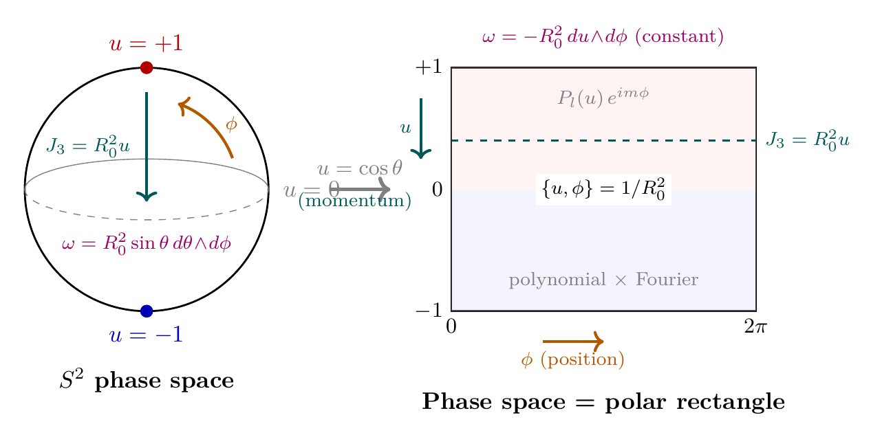
Polar verification: In the polar field variable $u = \cos\theta$, the symplectic form becomes the constant-coefficient Darboux form $\omega = -R_0^2\,du\wedge d\phi$, revealing that the $S^2$ phase space IS the flat rectangle $[-1,+1]\times[0,2\pi)$ with canonical pair $(u,\phi)$ satisfying $\{u,\phi\}=1/R_0^2$. The $z$-angular momentum $J_3 = R_0^2 u$ is linear in the polar variable, and the mode decomposition factorizes as polynomial (THROUGH) $\times$ Fourier (AROUND) on the flat domain (Figure fig:ch58-polar-phase-space).

Table 64.2: Chapter 58 results summary

Result	Value	Status	Reference
$S^2$ symplectic	$\omega=R_0^2\sin\theta\,d\theta\wedge d\phi$	ESTABLISHED	Thm thm:P3-Ch58-symplectic
Momentum map	$\mu=R_0^2\hat{x}$	PROVEN	Thm thm:P3-Ch58-momentum-map
$SO(3)$ conservation	$\{J_a,\mathcal{H}\}=0$	ESTABLISHED	Thm thm:P3-Ch58-noether
Mode spectrum	$E_l=l(l+1)/(2R_0^2)$	PROVEN	Thm thm:P10-Ch58-spectrum
Phase space $\to$ 4D	Table tab:ch58-dynamics-physics	PROVEN	\Ssec:ch58-momentum-maps
Polar symplectic	$\omega = -R_0^2\,du\wedge d\phi$ (constant)	PROVEN	\Ssec:ch58-polar-symplectic
Polar $J_3$	$J_3 = R_0^2 u$ (linear)	PROVEN	\Ssec:ch58-polar-momentum-map
Polar modes	$P_l^{\|m\|}(u)\,e^{im\phi}$ (poly $\times$ Fourier)	PROVEN	\Ssec:ch58-polar-modes

Verification Code

The mathematical derivations and proofs in this chapter can be independently verified using the formal and computational scripts below.

◆ Lean 4 Formal proof verification Coming Soon ● Python Numerical verification & plots Coming Soon ★ Mathematica Symbolic computation & CAS verification Coming Soon

All verification code is open source. See the complete verification index for all chapters.

Property	Spherical \((\theta, \phi)\)	Polar \((u, \phi)\)
Symplectic form	\(R_0^2\sin\theta\,d\theta\wedge d\phi\)	\(-R_0^2\,du\wedge d\phi\)
Coefficient	\(R_0^2\sin\theta\) (variable)	\(R_0^2\) (constant)
Area element	\(\sin\theta\,d\theta\,d\phi\) (curved)	\(du\,d\phi\) (flat)
Position variable	\(\phi \in [0,2\pi)\)	\(\phi \in [0,2\pi)\)
Momentum variable	\(\cos\theta\) (implicit)	\(u\) (explicit)
Canonical bracket	\(\\cos\theta,\phi\ = 1/R_0^2\)	\(\{u,\phi\} = 1/R_0^2\)
Total volume	\(\int\sin\theta\,d\theta\,d\phi\)	\(\int du\,d\phi = 4\pi\)

\(l\)	Modes	Energy	Physical Role
0	1	0	Modulus (size of \(S^2\))
1	3	\(1/R_0^2\)	Gauge modes (absorbed into \(SU(2)\))
\(2\)–\(11\)	140	\(3/R_0^2\) to \(66/R_0^2\)	Stiffness modes
\(\geq 12\)	—	\(\geq 78/R_0^2\)	Truncated by topological cutoff

\(l\)	THROUGH (polynomial)	AROUND (Fourier)	Physical Role
0	\(P_0(u) = 1\) (constant)	\(m = 0\) only	Modulus (uniform on rectangle)
1	\(P_1(u) = u\) (linear)	\(m = 0, \pm 1\)	Gauge (\(u\)-gradient + winding)
\(2\)–\(11\)	\(P_l(u)\) (degree \(l\))	\(\|m\| \leq l\)	Stiffness (polynomial \(\times\) Fourier)

Component	Spherical	Polar	Character	Physical Role
\(J_3\)	\(R_0^2\cos\theta\)	\(R_0^2 u\) (linear)	Pure THROUGH	Unbroken \(U(1)_{\mathrm{em}}\)
\(J_1\)	\(R_0^2\sin\theta\cos\phi\)	\(R_0^2\sqrt{1{-}u^2}\cos\phi\)	Mixed T\(\times\)A	Broken \(W^\pm\) (real)
\(J_2\)	\(R_0^2\sin\theta\sin\phi\)	\(R_0^2\sqrt{1{-}u^2}\sin\phi\)	Mixed T\(\times\)A	Broken \(W^\pm\) (imag)
\(\|\mathbf{J}\|^2\)	\(R_0^4\)	\(R_0^4\)	Casimir	Conserved magnitude

Classical Dynamics on S²

Introduction

Phase Space on the Compact Manifold

The Round \(S^2\) as a Symplectic Manifold

Polar Field Form of the Symplectic Structure

Phase Space Coordinates

The Classical Hamiltonian on \(S^2\)

Mode Decomposition and Energy Spectrum

Polar Mode Decomposition: Polynomial \(\times\) Fourier

Phase Space Volume and Quantization

Momentum Maps and Conservation

The \(SO(3)\) Action on \(S^2\)

Killing Vectors as Hamiltonian Vector Fields

Polar Field Form of the Momentum Map

Conservation Laws from Isometries

Physical Significance for TMT

Chapter Summary

Verification Code

\(S^2\) Structure	4D Physics	Source
Isometry \(SO(3)\)	\(SU(2)\) gauge symmetry	Part 3 \S7
Killing vectors \(\xi_a\)	Gauge fields \(A_\mu^a\)	Part 3 \S7.4
Momentum map \(J_a\)	Conserved charges	This chapter
Mode spectrum \(E_l\)	Particle/stiffness modes	Part 5 \S22
Symplectic volume \(4\pi R_0^2\)	\((D\chi)^2=144\) states	Part 5 \S22.3

Result	Value	Status	Reference
\(S^2\) symplectic	\(\omega=R_0^2\sin\theta\,d\theta\wedge d\phi\)	ESTABLISHED	Thm thm:P3-Ch58-symplectic
Momentum map	\(\mu=R_0^2\hat{x}\)	PROVEN	Thm thm:P3-Ch58-momentum-map
\(SO(3)\) conservation	\(\{J_a,\mathcal{H}\}=0\)	ESTABLISHED	Thm thm:P3-Ch58-noether
Mode spectrum	\(E_l=l(l+1)/(2R_0^2)\)	PROVEN	Thm thm:P10-Ch58-spectrum
Phase space \(\to\) 4D	Table tab:ch58-dynamics-physics	PROVEN	\Ssec:ch58-momentum-maps
Polar symplectic	\(\omega = -R_0^2\,du\wedge d\phi\) (constant)	PROVEN	\Ssec:ch58-polar-symplectic
Polar \(J_3\)	\(J_3 = R_0^2 u\) (linear)	PROVEN	\Ssec:ch58-polar-momentum-map
Polar modes	\(P_l^{\|m\|}(u)\,e^{im\phi}\) (poly \(\times\) Fourier)	PROVEN	\Ssec:ch58-polar-modes