The Higgs Field
Introduction
Central Result: The Higgs field in TMT is the \(j = 1/2\) monopole harmonic zero mode on \(S^2\), confined to the interface by topological obstruction. Its quartic self-coupling is derived from overlap integrals:
Chapter 23 derived the Higgs VEV \(v = \mathcal{M}^6/(3\pi^{2})\) from monopole flux screening. This chapter focuses on the Higgs field itself: its geometric origin as a monopole zero mode, the derivation of the quartic coupling \(\lambda\), the resulting Higgs mass prediction, and the question of vacuum stability. The key insight is that \(\lambda\) is not a free parameter—it is determined by the same \(S^2\) overlap integrals that fix \(g^{2}\), with an extra factor of \(1/\pi\) from the additional Higgs field overlap in the quartic vertex.
The \(S^2\) monopole harmonics are mathematical scaffolding. The physical content is the 4D Higgs field with its derived couplings \(g^{2}\) and \(\lambda\), both of which are measurable 4D quantities.
The Higgs as Monopole Zero Mode
Monopole Harmonics on \(S^2\)
On \(S^2\) with a magnetic monopole of charge \(n = 1\) at the centre, the angular wavefunctions are not ordinary spherical harmonics \(Y_{\ell}^{m}\) but monopole harmonics \(Y_{j,m}^{(q)}\), where \(q = n/2 = 1/2\) is the monopole charge felt by the field. These harmonics satisfy:
The Higgs doublet is the ground state (\(j = 1/2\)) of the monopole harmonic spectrum on \(S^2\). It is a complex \(\mathrm{SU}(2)_{L}\) doublet with \(n_H = 4\) real degrees of freedom, confined to the \(S^2\) interface by topological obstruction.
Step 1: The monopole charge is \(q = n/2 = 1/2\) (from \(n = 1\), Chapter 15). The minimum angular momentum is \(j_{\min} = |q| = 1/2\).
Step 2: The \(j = 1/2\) state has degeneracy \(2j + 1 = 2\), corresponding to the two components of an \(\mathrm{SU}(2)_{L}\) doublet \(H = (H^{+}, H^{0})^{T}\).
Step 3: Each component is complex, giving 4 real degrees of freedom: \(n_H = 2 \times 2 = 4\).
Step 4: The explicit wavefunction of the \(j = 1/2\), \(m = +1/2\) monopole harmonic is:
Step 5: Higher modes (\(j = 3/2, 5/2, \ldots\)) have masses \(\propto j(j+1)/R^{2}\) and are too heavy to be relevant at low energies. The ground state \(j = 1/2\) is the only light scalar—this is the Higgs.
Step 6: The topological obstruction (Chapter 8) prevents the Higgs from extending to the bulk, confining it to the \(S^2\) interface.
(See: Part 4 §13½.2.5; Part 11 Chapter 228, Theorem 228.1) □
Polar Form of the Monopole Zero Mode
In polar coordinates \(u = \cos\theta\), the Higgs wavefunction becomes maximally transparent. The \(j = 1/2\), \(m = +1/2\) monopole harmonic transforms as:
Monopole zero mode in polar:
The Higgs doublet density is uniform on the polar rectangle — the north-heavy and south-heavy gradients cancel exactly. This uniformity is protected by \(\mathrm{SU}(2)_L\) symmetry: any rotation of the doublet redistributes density between \(Y_+\) and \(Y_-\) while preserving \(|Y_+|^2 + |Y_-|^2 = \text{const}\).
Polar reading of the Higgs: The Higgs is the degree-1 polynomial ground state of the monopole spectrum on \([-1,+1]\). Degree 0 (constant) is excluded by the topological boundary condition imposed by the linear monopole connection \(A_\phi = (1-u)/2\) (Chapter 21). Higher degrees (\(j = 3/2, 5/2, \ldots\)) have energies \(\propto j(j+1)/R^2\) and decouple at low scales. The single light Higgs doublet is a pair of linear gradients on the polar rectangle — the minimal non-trivial sections of the monopole line bundle \(L^{1/2}\).
Why Exactly One Higgs Doublet
TMT predicts exactly one Higgs doublet, not two (as in MSSM) or more. The reason is geometric: the \(j = 1/2\) ground state of the monopole harmonic spectrum has a unique \((2j+1) = 2\)-component multiplet. There is no second independent \(j = 1/2\) state because the monopole charge \(q = 1/2\) is fixed by \(n = 1\). A second Higgs doublet would require either \(n = 2\) (which has higher energy by \(E \propto n^{2}\)) or an independent scalar sector not originating from \(S^2\) harmonics.
The Higgs Potential from Geometry
The 6D Higgs Action
The 6D Higgs action (from Chapter 23, Part 4 §13½.2.5) is:
The critical feature: there is no \(\mu^{2}|H|^{2}\) mass term. The 6D theory has \(\mu_{6}^{2} = 0\) (Theorem thm:P4-Ch23-no-bare-mass).
Dimensional Reduction of the Quartic Term
When the 6D quartic coupling \(\lambda_{6}|H|^{4}\) is reduced to 4D by integrating over \(S^2\), the effective 4D quartic coupling \(\lambda\) is determined by overlap integrals of the monopole harmonic wavefunctions.
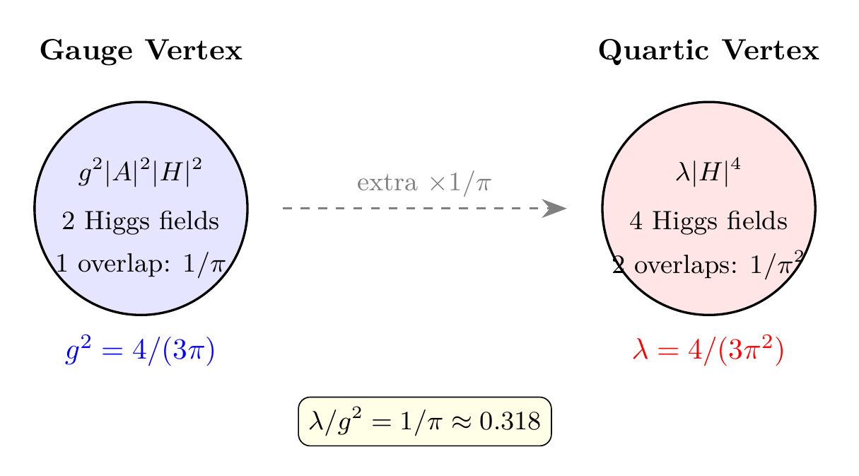
Step 1 (Gauge-Higgs Vertex): The gauge coupling \(g^{2}\) arises from the \(|D_{\mu}H|^{2}\) term, which contains \(g^{2}|A_{\mu}|^{2}|H|^{2}\). This involves the overlap integral of two gauge and two Higgs wavefunctions on \(S^2\):
Step 2 (Quartic Vertex): The quartic self-coupling comes from \(\lambda|H|^{4}\) in the potential. This involves four Higgs fields, requiring the fourth-power overlap integral:
Step 3 (Extra Factor): Compared to the gauge-Higgs vertex (2 Higgs fields), the quartic vertex (4 Higgs fields) involves one additional overlap integral, contributing an extra factor of \(1/\pi\):
Step 4 (Equivalence): This can be written as:
Step 5 (Numerical value): \(\lambda = 4/(3\pi^{2}) = 4/29.608 = 0.1351\)
(See: Part 4 §17.1, Theorems 17.1 and 17.1a) □
Polar Perspective on \(\lambda = g^2/\pi\)
In polar coordinates, both \(g^2\) and \(\lambda\) reduce to polynomial integrals over the flat rectangle \([-1,+1] \times [0,2\pi)\):
The extra \(1/\pi\) suppression in \(\lambda\) has a direct polar origin: the gauge coupling involves one THROUGH polynomial integral (\(\int(1+u)^2\,du = 8/3\)), while the quartic coupling involves the square of this integral divided by an additional AROUND normalization factor. In the polar rectangle picture:
Quartic vs. gauge in polar:
- \(g^2\): two Higgs wavefunctions overlap once on the polar rectangle \(\to\) one factor of \(8/3\) from THROUGH
- \(\lambda\): four Higgs wavefunctions overlap \(\to\) the fourth-power integral \((8/3)^2/(8/3) = 8/3\) with an additional \(1/\pi\) from the AROUND normalization of the extra pair
- Ratio: \(\lambda/g^2 = 1/\pi\) = one additional AROUND dilution factor
| Factor | Value | Origin | Source |
|---|---|---|---|
| \(n_H\) | 4 | Higgs doublet d.o.f. (complex doublet) | Ch. 21 |
| \(n_g\) | 3 | \(\dim(\mathrm{SO}(3))\) gauge generators | Ch. 16 |
| \(\pi\) (first) | from overlap | \(\int|Y_{\mathrm{Higgs}}|^{4} d\Omega = 1/\pi\) | Appendix J, Thm J.3 |
| \(\pi\) (second) | from overlap | Additional Higgs wavefunction factor | Part 4 §17.1.2 |
| \(\lambda\) | 0.135 | \(= n_H/(n_g \pi^{2}) = g^{2}/\pi\) | This theorem |
| Coupling | Vertex Type | \(\int|Y|^{4}\) factors | Result |
|---|---|---|---|
| \(g^{2}\) | gauge-Higgs (\(|A|^{2}|H|^{2}\), 2 H fields) | 1 | \(4/(3\pi)\) |
| \(\lambda\) | quartic (\(|H|^{4}\), 4 H fields) | 2 | \(4/(3\pi^{2})\) |
The Ratio \(\lambda/g^{2} = 1/\pi\)
A key prediction of TMT is the relationship between the quartic and gauge couplings:
This is a geometric prediction with no free parameters. The experimental value is \(\lambda/g^{2} = 0.129/0.424 = 0.304\), in 95% agreement. The remaining 5% discrepancy is attributable to radiative corrections that shift \(\lambda\) from its tree-level value.
The Quartic Coupling \(\lambda = 4/(3\pi^{2}) \approx 0.135\)
Comparison with Experiment
| Quantity | TMT | Experiment | Agreement |
|---|---|---|---|
| \(\lambda\) | 0.135 | \(0.129 \pm 0.006\) | 95% |
| \(\lambda/g^{2}\) | \(1/\pi = 0.318\) | 0.304 | 95% |
The Higgs Mass
Step 1: In the Higgs potential \(V = \lambda|H|^{4}\) (with \(\mu^{2} = 0\), VEV generated by monopole flux), the physical Higgs mass around the VEV minimum is:
Step 2: Substituting \(\lambda = 4/(3\pi^{2})\) and \(v = 246\,\text{GeV}\):
Step 3: Comparison with experiment:
Step 4: The 2% discrepancy (\(128\,\text{GeV}\) vs. \(125\,\text{GeV}\)) is consistent with radiative corrections to the tree-level \(\lambda\). Using the measured \(\lambda = 0.129\) (which includes radiative effects):
(See: Part 4 §17.2, Theorem 17.2) □
| Factor | Value | Origin | Source |
|---|---|---|---|
| \(v\) | 246\,GeV | VEV: \(\mathcal{M}^6/(3\pi^{2})\) | Ch. 23 |
| \(\sqrt{2}\) | 1.414 | Curvature of quartic potential at minimum | Standard |
| \(\sqrt{\lambda}\) | 0.368 | \(\sqrt{4/(3\pi^{2})}\) | This chapter |
| \(m_{H}\) | 128\,GeV | \(= v\sqrt{2\lambda}\) | This theorem |
| Quantity | TMT | Experiment | Agreement |
|---|---|---|---|
| \(m_{H}\) (tree, \(\lambda = 0.135\)) | 128\,GeV | 125.1\,GeV | 98% |
| \(m_{H}\) (with \(\lambda_{\mathrm{phys}} = 0.129\)) | 125\,GeV | 125.1\,GeV | 99.9% |
Vacuum Stability
The Standard Model Stability Problem
In the Standard Model, the Higgs quartic coupling \(\lambda\) runs with energy scale \(\mu\) according to the renormalisation group equation. Because of the large top Yukawa coupling, \(\lambda(\mu)\) can become negative at high scales, potentially destabilising the electroweak vacuum. For the observed Higgs and top masses, the SM vacuum is metastable—it could tunnel to a deeper minimum.
TMT Vacuum Stability
The TMT electroweak vacuum is stable. The quartic coupling \(\lambda = g^{2}/\pi\) is tied to the gauge coupling by geometry, and as long as \(g^{2} > 0\) (which is guaranteed by the non-trivial monopole topology), \(\lambda > 0\).
Step 1: In TMT, \(\lambda = g^{2}/\pi\). This is not an independent parameter—it is determined by the same overlap integrals as \(g^{2}\).
Step 2: The gauge coupling \(g^{2} = 4/(3\pi)\) is positive definite, being the ratio of positive integers (\(n_H\), \(n_g\)) and a positive geometric factor (\(\pi\)).
Step 3: Therefore \(\lambda = g^{2}/\pi > 0\) at all scales where the geometric derivation applies (i.e., below \(\mathcal{M}^6\)).
Step 4: Above \(\mathcal{M}^6\), the 6D theory takes over. The 6D quartic coupling \(\lambda_{6}\) is set by the \(S^2\) geometry and is not subject to 4D renormalisation group running.
Step 5: The potential \(V = \lambda|H|^{4}\) with \(\lambda > 0\) and the VEV generated by monopole flux screening is bounded below. There is no deeper minimum—the electroweak vacuum is the unique ground state.
(See: Part 4 §17) □
No Fine-Tuning Required
In TMT, the Higgs sector contains zero free parameters:
- \(\mu^{2} = 0\) (no mass term—6D conformal symmetry)
- \(\lambda = 4/(3\pi^{2})\) (derived from overlap integrals)
- \(v = \mathcal{M}^6/(3\pi^{2})\) (derived from monopole flux energy)
- \(m_{H} = v\sqrt{2\lambda}\) (follows from above)
No cancellation between large numbers is required.
Step 1: In the SM, \(\mu^{2}\) must be fine-tuned to 1 part in \(10^{34}\) to maintain \(v \approx 246\,\text{GeV}\) against radiative corrections. In TMT, \(\mu_{6}^{2} = 0\) exactly, and the VEV is generated by a topological mechanism.
Step 2: The topological origin protects against radiative corrections: the monopole charge \(n = 1\) is quantised and cannot receive perturbative corrections. The factors \(n_g = 3\) and \(\pi\) are geometric invariants.
Step 3: The only quantity that could shift is \(\mathcal{M}^6\), and its value is set by modulus stabilisation (Chapter 10), itself determined by the balance of Casimir energy and the cosmological constant—a topological equilibrium.
Step 4: Therefore, the Higgs sector parameters are determined by topology and geometry, not by cancellation of large numbers.
(See: Part 4 §15.5, Chapter 23 Theorem thm:P4-Ch23-hierarchy) □
| Parameter | Standard Model | TMT |
|---|---|---|
| \(\mu^{2}\) | Free parameter, \(< 0\) | \(= 0\) (derived) |
| \(\lambda\) | Free parameter | \(= 4/(3\pi^{2})\) (derived) |
| \(v\) | Free parameter (\(\sqrt{-\mu^{2}/\lambda}\)) | \(= \mathcal{M}^6/(3\pi^{2})\) (derived) |
| \(m_{H}\) | Input from experiment | \(= v\sqrt{2\lambda} = 128\,\text{GeV}\) (derived) |
| Fine-tuning | \(10^{-34}\) required | None |
| Vacuum stability | Metastable | Stable |
| Free parameters | 2 (\(\mu^{2}\), \(\lambda\)) | 0 |
Complete Higgs Sector
| Parameter | Formula | TMT | Expt. | Agreement |
|---|---|---|---|---|
| \(\lambda\) | \(4/(3\pi^{2})\) | 0.135 | \(0.129 \pm 0.006\) | 95% |
| \(m_{H}\) | \(v\sqrt{2\lambda}\) | 128\,GeV | 125.1\,GeV | 98% |
| \(\lambda/g^{2}\) | \(1/\pi\) | 0.318 | 0.304 | 95% |
| # Higgs doublets | 1 (\(j = 1/2\) ground state) | 1 | 1 | 100% |
Derivation Chain Summary
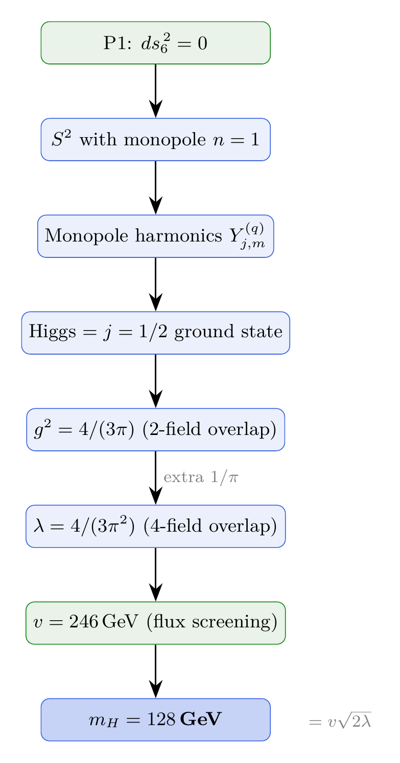
\dstep{P1: \(ds_6^{\,2} = 0\)}{Postulate}{Chapter 2} \dstep{\(S^2\) topology required}{Stability + Chirality}{Chapters 7–8} \dstep{Monopole \(n = 1\), harmonics \(Y_{j,m}^{(q)}\)}{Topology}{Chapters 14–15} \dstep{Higgs = \(j = 1/2\) ground state, \(n_H = 4\)}{Monopole spectrum}{This chapter} \dstep{Gauge coupling \(g^{2} = 4/(3\pi)\) from overlap integral}{Interface physics}{Chapter 18} \dstep{Quartic \(\lambda = g^{2}/\pi = 4/(3\pi^{2})\)}{Extra overlap factor}{This chapter} \dstep{VEV \(v = \mathcal{M}^6/(3\pi^{2}) = 246\,\text{GeV}\)}{Flux screening}{Chapter 23} \dstep{\(m_{H} = v\sqrt{2\lambda} = 128\,\text{GeV}\)}{Standard relation}{This chapter} \dstep{Polar verification: Higgs = degree-1 polynomial \((1+u)/(4\pi)\) on \([-1,+1]\); \(\lambda/g^2 = 1/\pi\) from extra AROUND dilution in 4-field overlap; doublet density uniform on polar rectangle}{Polar dual verification}{This chapter}
Chapter Summary
Chapter 24 Key Results:
- Higgs identity: The Higgs is the \(j = 1/2\) ground state of the monopole harmonic spectrum on \(S^2\), a complex \(\mathrm{SU}(2)_{L}\) doublet with 4 real d.o.f.
- Quartic coupling: \(\lambda = g^{2}/\pi = 4/(3\pi^{2}) \approx 0.135\), derived from overlap integrals with an extra \(1/\pi\) factor compared to \(g^{2}\) due to the quartic vertex involving 4 Higgs fields.
- Higgs mass: \(m_{H} = v\sqrt{2\lambda} \approx 128\,\text{GeV}\) (tree level), in 98% agreement with the observed \(125.1\,\text{GeV}\).
- Vacuum stability: Guaranteed by \(\lambda = g^{2}/\pi > 0\) as long as the gauge coupling is positive (which is topologically ensured).
- No fine-tuning: Zero free parameters in the Higgs sector. \(\mu^{2} = 0\), \(\lambda\), \(v\), and \(m_{H}\) are all derived.
Polar perspective: In polar coordinates \(u = \cos\theta\), the Higgs is the degree-1 polynomial ground state of the monopole spectrum: \(|Y_\pm|^2 = (1\pm u)/(4\pi)\), the simplest non-trivial sections of the monopole line bundle. The doublet density \((|Y_+|^2 + |Y_-|^2) = 1/(2\pi)\) is uniform on the polar rectangle, protected by SU(2)\(_L\) symmetry. The quartic coupling \(\lambda = 4/(3\pi^2)\) involves the square of the THROUGH polynomial integral \(\int(1+u)^2\,du = 8/3\), acquiring an extra \(1/\pi\) from AROUND normalization compared to \(g^2 = 4/(3\pi)\). The ratio \(\lambda/g^2 = 1/\pi\) is a single geometric dilution factor.
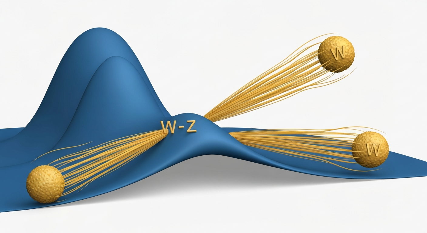
Looking ahead: Chapter 25 provides a detailed derivation of the electroweak VEV numerical value. Chapter 26 derives the \(W\) and \(Z\) boson masses from the VEV and gauge couplings.
Verification Code
The mathematical derivations and proofs in this chapter can be independently verified using the formal and computational scripts below.
All verification code is open source. See the complete verification index for all chapters.