Monopole Harmonics
Ordinary Spherical Harmonics \(Y_{\ell m}\)
Before developing the monopole harmonics, we recall the ordinary spherical harmonics on \(S^2\)—the eigenfunctions of the scalar Laplacian without a monopole background (\(q = 0\)).
The scalar Laplacian on \(S^2\) with radius \(R\) is (Chapter 9):
The ordinary spherical harmonics \(Y_{\ell m}(\theta,\phi)\) satisfy:
with degeneracy \(2\ell + 1\) for each \(\ell\). These are the standard functions used in quantum mechanics for angular momentum eigenstates.
Key distinction: Ordinary harmonics apply to uncharged fields (\(q = 0\)) that propagate THROUGH \(S^2\), such as the graviton and the modulus. For charged fields (\(q \neq 0\)) that are sections of the monopole bundle, we need the monopole harmonics developed below.
Monopole Harmonics \(Y_{qlm}\)
In the presence of a Dirac monopole with charge \(n\), a particle with charge \(q\) satisfying the Dirac condition \(qn \in \mathbb{Z}\) moves on \(S^2\) under the influence of the monopole gauge field. The eigenfunctions of the covariant Laplacian in this background are the monopole harmonics \(Y^{(q)}_{j,m}\).
The Covariant Derivative
For a field \(\psi\) with charge \(q\) on \(S^2\) with a monopole of charge \(n = 1\):
Explicitly (northern patch, \(n = 1\), \(q = 1/2\)):
The key point: \(A_\theta = 0\) in both patches, so \(D_\theta = \partial_\theta\). Only the \(\phi\)-component is modified.
The Covariant Laplacian
Step 1: The covariant Laplacian is defined as:
Step 2: Using \(\sqrt{g} = R^2\sin\theta\) and the inverse metric \(g^{ab}\):
For \(a = \theta\):
For \(a = \phi\):
Step 3: Combining with the overall \(1/R^2\) factor:
(See: Part 2 App 2A) □
The eigenvalue problem is:
Dimension check: \([\lambda] = [1/R^2] = [\text{Length}^{-2}]\) \checkmark.
The Monopole Charge \(q\)
The charge \(q\) controls the coupling of a field to the monopole background. From Chapter 10:
- \(q = 0\): Uncharged field. Ordinary Laplacian, ordinary spherical harmonics. Field propagates THROUGH.
- \(q = 1/2\): Minimal half-integer charge (Higgs). Section of spin\(^c\) bundle. Field lives ON the interface.
- \(q = 1\): Integer charge. Standard monopole harmonic.
For TMT, the physically relevant case is \(q = 1/2\) (the Higgs field in the monopole background with \(n = 1\)). All subsequent derivations specialize to this case.
The action for a charged scalar on \(S^2\) is:
Expanding explicitly:
Variation \(\delta S/\delta\psi^* = 0\) gives the equation of motion \(-D^2_{S^2}\psi = 0\), and with an eigenvalue: \(-D^2_{S^2}\psi = \lambda\psi\).
Selection Rules
Separation of Variables
Ansatz: Since \(A_\phi\) is independent of \(\phi\), we separate:
For the \(\phi\)-dependence, try \(\Phi(\phi) = e^{i\mu\phi}\) where \(\mu\) is to be determined.
For \(q = 1/2\), \(n = 1\): the magnetic quantum number \(m = \mu\) must be half-integer:
This follows from the anti-periodicity requirement: \(\psi(\phi + 2\pi) = -\psi(\phi)\) for sections of the \(q = 1/2\) bundle (Chapter 10, Theorem thm:P2-Ch10-half-integer).
Angular Momentum Operators
Define the covariant angular momentum:
The total angular momentum squared for monopole harmonics is:
This definition ensures that sections with charge \(q\) form representations of SU(2) with:
The selection rule \(j \geq |q|\) follows from the representation theory of SU(2) acting on sections of the line bundle.
Orthogonality and Completeness
The monopole harmonics form a complete orthonormal set on \(S^2\):
Completeness:
These properties are standard results from the representation theory of SU(2) acting on sections of line bundles over \(S^2\).
Role in Fermion Wavefunctions
Fermions in the TMT framework are described by spinor-valued sections of the monopole bundle. Their wavefunctions on \(S^2\) are expanded in monopole harmonics:
where \(\psi_{j,m}(x^\mu)\) are 4D spinor fields and \(Y^{(q)}_{j,m}\) are the monopole harmonics with the appropriate charge \(q\).
The ground state (\(j = |q|\)) modes are the lightest and dominate at low energies. Higher modes (\(j > |q|\)) are heavier by factors of \(1/R^2\) and are excited only at energies above the compactification scale.
For the Higgs (\(q = 1/2\)), the ground state \(j = 1/2\) doublet gives exactly the Standard Model Higgs field, with heavier modes forming a “Kaluza-Klein tower” that is too heavy to be observed at current energies.
Killing Vectors on \(S^2\)
The isometry group SO(3) of \(S^2\) is generated by three Killing vector fields. These vector fields play a dual role: they generate the gauge symmetry (Chapter 9) and they define the angular momentum operators for monopole harmonics.
SO(3) Generators \(\xi_1, \xi_2, \xi_3\)
The Killing equation on \(S^2\) requires \(\nabla_{(a}\xi_{b)} = 0\). For \(\xi_3 = \partial_\phi\): this is manifest since the metric \(ds^2 = d\theta^2 + \sin^2\theta\, d\phi^2\) is independent of \(\phi\).
For \(\xi_1\) and \(\xi_2\): these are the infinitesimal generators of rotations about the \(x\) and \(y\) axes respectively, obtained from the standard embedding \(S^2 \hookrightarrow \mathbb{R}^3\) (Chapter 9). The Killing equation can be verified by direct computation of the covariant derivatives.
(See: Part 2 App 2A.1) □
Commutation Relations
The Killing vectors satisfy the SO(3) Lie algebra with the standard sign convention for right-action generators:
Explicitly:
(The minus sign is the standard convention: Killing vectors on \(S^2\) generate right-action rotations, giving \([\xi_a, \xi_b] = -\epsilon_{abc}\xi_c\). The quantum angular momentum operators \(L_a = -i\xi_a\) then satisfy \([L_a, L_b] = i\epsilon_{abc}L_c\).)
All three commutators are verified by direct computation using the Lie bracket \([\xi_a, \xi_b](f) = \xi_a(\xi_b(f)) - \xi_b(\xi_a(f))\).
Step 1 (\([\xi_1, \xi_2] = -\xi_3\)): We compute the \(\theta\) and \(\phi\) components of \([\xi_1, \xi_2]\) using \([\xi_a, \xi_b]^i = \xi_a^j \partial_j \xi_b^i - \xi_b^j \partial_j \xi_a^i\).
\(\partial_\theta\) coefficient:
\(\partial_\phi\) coefficient:
Therefore \([\xi_1, \xi_2] = -\partial_\phi = -\xi_3\). \checkmark
Step 2 (\([\xi_2, \xi_3] = -\xi_1\)): Since \(\xi_3 = \partial_\phi\) has constant coefficients, \(\xi_2^j \partial_j \xi_3^i = 0\). The commutator reduces to:
Therefore \([\xi_2, \xi_3] = \sin\phi\,\partial_\theta + \cos\phi\cot\theta\,\partial_\phi\). Since \(\xi_1 = -\sin\phi\,\partial_\theta - \cos\phi\cot\theta\,\partial_\phi\), we have \([\xi_2, \xi_3] = -\xi_1\). \checkmark
Step 3 (\([\xi_3, \xi_1] = -\xi_2\)): Again \(\xi_3 = \partial_\phi\) has constant coefficients, so:
Therefore \([\xi_3, \xi_1] = -\cos\phi\,\partial_\theta + \sin\phi\cot\theta\,\partial_\phi\). Since \(\xi_2 = \cos\phi\,\partial_\theta - \sin\phi\cot\theta\,\partial_\phi\), we have \([\xi_3, \xi_1] = -\xi_2\). \checkmark
All three commutation relations are verified. The algebra is \(\mathfrak{so}(3)\) with structure constants \(f_{ijk} = -\epsilon_{ijk}\).
(See: Part 2 App 2A.1) □
Killing Vector Norms
On the unit \(S^2\) (with metric \(g_{\theta\theta} = 1\), \(g_{\phi\phi} = \sin^2\theta\)), the pointwise norms \(|\xi|^2 = g_{ab}\xi^a\xi^b\) are:
These vary individually over \(S^2\), but the Casimir invariant is constant:
Step 1 (\(|\xi_1|^2\)): With \(\xi_1 = -\sin\phi\,\partial_\theta - \cos\phi\cot\theta\,\partial_\phi\):
Step 2 (\(|\xi_2|^2\)): With \(\xi_2 = \cos\phi\,\partial_\theta - \sin\phi\cot\theta\,\partial_\phi\):
Step 3 (\(|\xi_3|^2\)): With \(\xi_3 = \partial_\phi\):
Step 4 (Casimir sum):
The constancy of the Casimir reflects the underlying SO(3) symmetry: the sum over a complete basis of Killing vectors is a rotationally invariant tensor, hence proportional to the metric, and the trace gives a constant.
Integrated norms (used in gauge coupling derivations):
(See: Part 2 App 2A.1) □
Eigenvalue Spectrum
Separation of Variables
Ansatz: \(\psi(\theta, \phi) = \Theta(\theta) \cdot e^{im\phi}\) with \(m\) half-integer for \(q = 1/2\).
Substituting into the eigenvalue equation \(-D^2_{S^2}\psi = \lambda\psi\) and using the change of variables \(u = \cos\theta\), the \(\theta\)-equation becomes a form of the Jacobi differential equation. The regularity conditions at both poles (\(\theta = 0\) and \(\theta = \pi\)) select the eigenvalue:
where \(j = |q| + n_r\) for non-negative integer \(n_r = 0, 1, 2, \ldots\) (the radial quantum number on \(S^2\)).
\(\lambda_j = [j(j+1) - q^2]/R^2\)
Step 1: Define the shifted angular momentum. The covariant Laplacian can be written in terms of angular momentum operators. Define:
Step 2: Define the Casimir operator. The total angular momentum squared for monopole harmonics is:
Step 3: From representation theory, sections with charge \(q\) form representations of SU(2) with \(j \geq |q|\), and:
Step 4: Solving for the eigenvalue of \(-D^2_{S^2}\):
Therefore \(\lambda_j = [j(j+1) - q^2]/R^2\).
(See: Part 2 App 2A) □
Constraint \(j \geq |q|\)
For the eigenvalue equation \(-D^2_{S^2}\psi = \lambda\psi\) with charge \(q\), we must have \(j \geq |q|\).
The operator \(-D^2_{S^2}\) is positive semi-definite (self-adjoint with non-negative inner products). Therefore:
This requires \(j(j+1) \geq q^2\). For \(j \geq 0\), the function \(f(j) = j(j+1)\) is increasing:
- At \(j = |q|\): \(f(|q|) = |q|(|q|+1) = q^2 + |q| > q^2\) \checkmark
- At \(j = |q| - 1\): \(f(|q|-1) = (|q|-1)|q| = q^2 - |q| < q^2\) ✗
So the minimum allowed value is \(j = |q|\).
(See: Part 2 App 2A) □
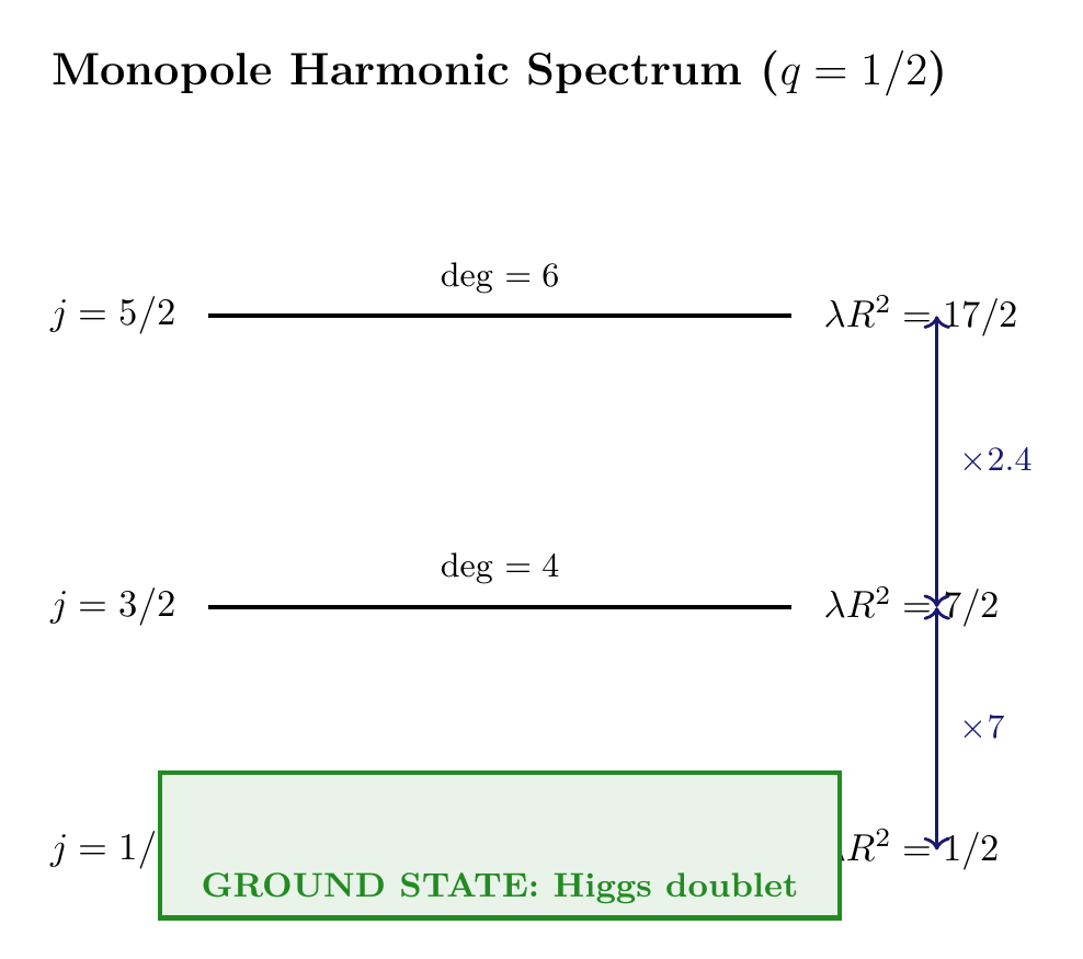
Spectrum Table (\(q = 1/2\))
For the physically relevant case \(q = 1/2\):
| \(j\) | \(\lambda R^2 = j(j+1) - 1/4\) | Numerical | Degeneracy \((2j+1)\) |
|---|---|---|---|
| \(1/2\) | \(3/4 - 1/4 = \mathbf{1/2}\) | 0.5 | 2 |
| \(3/2\) | \(15/4 - 1/4 = 7/2\) | 3.5 | 4 |
| \(5/2\) | \(35/4 - 1/4 = 17/2\) | 8.5 | 6 |
| \(7/2\) | \(63/4 - 1/4 = 31/2\) | 15.5 | 8 |
The ground state is \(j = 1/2\) with eigenvalue \(\lambda = 1/(2R^2)\) and degeneracy 2.
The ratio of the first excited state to the ground state is \(\lambda_{3/2}/\lambda_{1/2} = 7\), so the first excited mode is 7 times heavier. At energies below \(1/R\), only the ground state is relevant.
The Ground State
\(j = 1/2\), \(\lambda = 1/(2R^2)\)
For a charge \(q = 1/2\) field on \(S^2\) with a monopole (\(n = 1\)):
- Ground state angular momentum: \(j = 1/2\)
- Ground state eigenvalue: \(\lambda = 1/(2R^2)\)
- Ground state degeneracy: 2 (states \(m = +1/2\) and \(m = -1/2\))
From Theorem thm:P2-Ch11-minimum-j, \(j \geq |q| = 1/2\). The minimum is \(j = 1/2\), which gives:
Degeneracy \(= 2j + 1 = 2\).
(See: Part 2 App 2A) □
Degeneracy \(= 2\)
The degeneracy 2 means there are exactly two linearly independent ground state wavefunctions, labeled by \(m = +1/2\) and \(m = -1/2\). These two complex states form an SU(2) doublet.
Physical interpretation: The ground state monopole harmonics on \(S^2\) with \(q = 1/2\) form a complex doublet—precisely the structure of the Standard Model Higgs field. This is not imposed but follows from the topology (\(n = 1\) monopole) and energy minimization (\(j = |q| = 1/2\)).
Physical Interpretation
Why \(j = 1/2\) is the ground state:
- Minimum angular momentum: The monopole field carries angular momentum \(q = 1/2\). The particle cannot have \(j < 1/2\) (Theorem thm:P2-Ch11-minimum-j).
- No angular nodes: Like an \(s\)-orbital in atoms (\(\ell = 0\)), the \(j = |q|\) state has the minimum angular structure compatible with the monopole background.
- Lowest energy: \(\lambda\) increases with \(j\), so \(j = |q|\) minimizes the eigenvalue.
Explicit \(j = 1/2\) Harmonics
\(\theta\)-Functions: \(\cos(\theta/2)\), \(\sin(\theta/2)\)
From solving the \(\theta\)-differential equation with regularity conditions at both poles:
For \(m = +1/2\): \(f_{+1/2}(\theta) = \cos(\theta/2)\)
For \(m = -1/2\): \(f_{-1/2}(\theta) = \sin(\theta/2)\)
These are the unique regular solutions. The half-angle functions arise because the charge \(q = 1/2\) creates half-integer angular momentum, requiring spinorial behavior.
Behavior at poles:
- \(f_{+1/2}(0) = \cos(0) = 1\), \(f_{+1/2}(\pi) = \cos(\pi/2) = 0\)
- \(f_{-1/2}(0) = \sin(0) = 0\), \(f_{-1/2}(\pi) = \sin(\pi/2) = 1\)
The \(m = +1/2\) state is concentrated near the north pole, the \(m = -1/2\) state near the south pole.
Normalization: \(N = 1/\sqrt{2\pi}\)
The normalization constant for both \(j = 1/2\) monopole harmonics is:
For \(Y_{+1/2}\):
Step 1: Write the normalization condition:
Step 2: Evaluate the \(\theta\) integral using \(\sin\theta = 2\sin(\theta/2)\cos(\theta/2)\):
Step 3: Substitute \(u = \cos(\theta/2)\), \(du = -\frac{1}{2}\sin(\theta/2)\, d\theta\):
Step 4: Combine with \(\phi\) integral:
By the symmetry \(\cos(\theta/2) \leftrightarrow \sin(\theta/2)\) (with the same integration measure), \(N_{-1/2} = 1/\sqrt{2\pi}\) as well.
(See: Part 2 App 2A) □
\(Y_{\pm 1/2} = \frac{1}{\sqrt{2\pi}}\{\cos,\sin\}(\theta/2)\,e^{\pm i\phi/2}\)
Three independent confirmations that \(Y_{\pm 1/2}\) are correct eigenfunctions:
- By construction: We solved the differential equation with regularity conditions at both poles. The solutions \(\cos(\theta/2)\) and \(\sin(\theta/2)\) emerge uniquely.
- By normalization consistency: The normalization integrals give exactly \(1/(2\pi)\), matching the completeness relation for \(j = 1/2\) monopole harmonics.
- By the uniformity identity: The sum \(|Y_{+1/2}|^2 + |Y_{-1/2}|^2 = 1/(2\pi)\) uses \(\cos^2(\theta/2) + \sin^2(\theta/2) = 1\), which is the fundamental Pythagorean identity for half-angle functions.
Polar Field Form: The Monopole Is a Linear Gradient
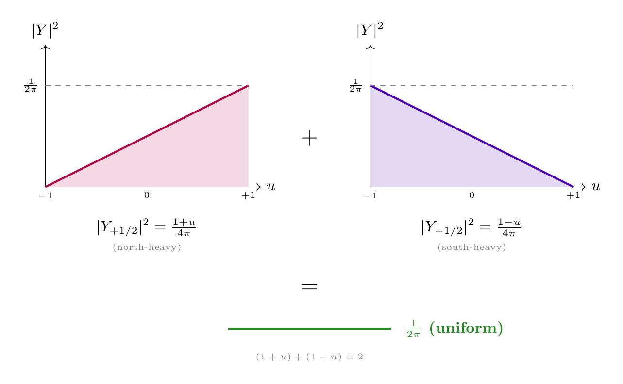
Using \(\cos^2(\theta/2) = (1 + \cos\theta)/2 = (1 + u)/2\) and \(\sin^2(\theta/2) = (1 - u)/2\), the probability densities become:
These are linear functions of \(u\) — the simplest possible non-trivial functions on \([-1, +1]\). The monopole harmonic densities are linear gradients in the polar field variable:
- \(Y_{+1/2}\): linearly increasing from \(0\) at south pole (\(u = -1\)) to \(1/(2\pi)\) at north pole (\(u = +1\))
- \(Y_{-1/2}\): linearly decreasing from \(1/(2\pi)\) at north pole to \(0\) at south pole
- Together: uniform density \(1/(2\pi)\) everywhere
Normalization verification (polar):
Compare with the spherical proof (Theorem thm:P2-Ch11-normalization): the substitution \(u = \cos(\theta/2)\), the factor \(\sin\theta = 2\sin(\theta/2)\cos(\theta/2)\), the integral \(4\int_0^1 u^3\,du = 1\) — all of that complexity was hiding a linear integral.
Physical insight: The monopole “tilts” the probability density from south to north (for \(Y_{+1/2}\)) or north to south (for \(Y_{-1/2}\)). In polar coordinates, this tilt is literally a straight line. The chiral asymmetry of the weak interaction reduces to the slope of a linear function on \([-1,+1]\).
Uniformity and the Participation Ratio
This section contains the key results that feed directly into the gauge coupling derivation.
Uniformity: \(|Y|^2 = 1/(2\pi)\)
Step 1: Compute \(|Y_{+1/2}|^2\):
Step 2: Compute \(|Y_{-1/2}|^2\):
Step 3: Sum:
The \(\phi\)-dependence has already cancelled (the modulus \(|e^{\pm i\phi/2}|^2 = 1\)). The \(\theta\)-dependence cancels via the Pythagorean identity. The result is a constant, uniform over \(S^2\).
(See: Part 2 App 2A) □
Uniformity from Symmetry
For any \(j = |q|\) multiplet, the sum \(\sum_m |Y_{j,m}|^2\) is uniform over \(S^2\).
Step 1: The sum over a complete multiplet transforms as a scalar under rotations (using unitarity of Wigner \(D\)-matrices).
Step 2: The only rotationally invariant function on \(S^2\) is a constant.
Step 3: The constant is determined by normalization:
If \(\sum_m |Y_{j,m}|^2 = C\) (constant), then \(C \cdot 4\pi = 2j + 1\), so:
For \(j = 1/2\): \(C = 2/(4\pi) = 1/(2\pi)\) \checkmark.
(See: Part 2 App 2A) □
Physical interpretation: Why \(1/(2\pi)\) and not \(1/(4\pi)\)?
- ONE state uniformly spread over \(S^2\): density \(= 1/(4\pi)\) per steradian.
- TWO states (the doublet), each normalized to 1, total integral \(= 2\).
- Uniform density \(\times\, 4\pi = 2\), therefore density \(= 2/(4\pi) = 1/(2\pi)\).
The factor of 2 in \(1/(2\pi)\) is the dimension of the \(j = 1/2\) representation (\(2j + 1 = 2\)).
Polar field verification: Using the polar densities from eq:ch11-polar-densities:
Fourth Moment: \(\int |Y|^4\, d\Omega = 1/\pi\)
From Theorem thm:P2-Ch11-uniformity: \(|Y|^2 = 1/(2\pi)\) (constant).
Step 1: Square the density:
Step 2: Integrate over \(S^2\):
(See: Part 2 App 2A) □
Expanding \(|Y|^4 = (|Y_{+1/2}|^2 + |Y_{-1/2}|^2)^2\) into three terms and integrating each over \(S^2\).
Throughout, we use the substitution \(u = \cos(\theta/2)\), \(du = -\frac{1}{2}\sin(\theta/2)\,d\theta\), with \(\sin\theta = 2\sin(\theta/2)\cos(\theta/2)\), so that \(\sin\theta\, d\theta = -4u\, du\) (limits: \(\theta = 0 \to u = 1\), \(\theta = \pi \to u = 0\)).
Term 1: \(\int_{S^2} |Y_{+1/2}|^4\, d\Omega\).
With \(|Y_{+1/2}|^2 = \frac{1}{2\pi}\cos^2(\theta/2)\) and the \(\phi\)-integral giving \(2\pi\):
Term 2: \(\int_{S^2} |Y_{-1/2}|^4\, d\Omega\).
By the substitution \(v = \sin(\theta/2)\) (or equivalently by \(\theta \to \pi - \theta\) symmetry): \(\int |Y_{-1/2}|^4\, d\Omega = \frac{1}{3\pi}\).
Cross term: \(2\int_{S^2} |Y_{+1/2}|^2|Y_{-1/2}|^2\, d\Omega\).
(Here we used \(\sin^2(\theta/2) = 1 - u^2\) and the measure \(\sin\theta\, d\theta = 4u\, du\).)
Total:
This confirms Method 1 by explicit integration. The equal splitting of \(1/\pi\) into three terms of \(1/(3\pi)\) each is a non-trivial consistency check.
(See: Part 2 App 2A) □
Using the polar densities eq:ch11-polar-densities and noting that the total density is constant:
For the individual fourth moments (which feed the coupling formula):
The crucial integral \(\int_{-1}^{+1}(1+u)^2\,du = 8/3\) gives the factor of 3 that appears in the coupling constant \(g^2 = 4/(3\pi)\). This factor has a transparent polar origin:
Participation Ratio \(P = \pi\)
The participation ratio \(P\) quantifies how spread out the wavefunction is on \(S^2\):
Physical meaning: \(P\) measures the effective solid angle over which the wavefunction participates:
- \(P = 4\pi\): maximally spread (uniform over entire sphere with unit normalization)
- \(P \to 0\): maximally localized (delta function)
Direct application of the definition with Theorem thm:P2-Ch11-fourth-moment:
(See: Part 2 App 2A) □
Physical interpretation: Why \(P = \pi\) and not \(4\pi\)?
For a SINGLE state uniformly spread over \(S^2\): \(P = 4\pi\).
For our DOUBLET with density \(1/(2\pi)\):
- Fourth moment \(= (1/(2\pi))^2 \times 4\pi = 1/\pi\)
- \(P = \pi\)
The factor of 4 difference comes from the density being \(2\times\) larger (two states instead of one). The doublet effectively “participates” over \(\pi\) steradians, which is \(1/4\) of the full sphere (\(4\pi\)).
Summary: Derived Results and Connection to Coupling
Derived Results Table
| Result | Formula | Section | Status |
|---|---|---|---|
| Eigenvalue equation | \(-D^2_{S^2}Y = \frac{j(j+1) - q^2}{R^2}Y\) | §sec:eigenvalue-spectrum | PROVEN |
| Minimum \(j\) | \(j \geq |q|\) | §sec:eigenvalue-spectrum | PROVEN |
| Ground state | \(j = 1/2\), \(\lambda = 1/(2R^2)\), deg \(= 2\) | §sec:ground-state | PROVEN |
| Explicit harmonics | \(Y_{\pm 1/2} = \frac{1}{\sqrt{2\pi}}\{\cos,\sin\}(\theta/2)\,e^{\pm i\phi/2}\) | §sec:explicit-harmonics | PROVEN |
| Uniformity | \(|Y|^2 = 1/(2\pi)\) | §sec:uniformity | PROVEN |
| Fourth moment | \(\int|Y|^4\, d\Omega = 1/\pi\) | §sec:uniformity | PROVEN |
| Participation ratio | \(P = \pi\) | §sec:uniformity | PROVEN |
Factor Origin Table
| Factor | Value | Origin | Reference |
|---|---|---|---|
| \(q = 1/2\) | 0.5 | Dirac quantization (min. half-integer) | Chapter 10 |
| \(j = 1/2\) | 0.5 | Minimum \(j = |q|\) from eigenvalue positivity | Thm thm:P2-Ch11-minimum-j |
| 2 (degeneracy) | 2 | \(2j + 1\) for \(j = 1/2\) | Thm thm:P2-Ch11-ground-state |
| \(1/\sqrt{2\pi}\) (normalization) | 0.399 | \(\int |Y|^2 d\Omega = 1\) over \(4\pi\) with 2 states | Thm thm:P2-Ch11-normalization |
| \(1/(2\pi)\) (density) | 0.159 | Two unit-normalized states over \(4\pi\) area | Thm thm:P2-Ch11-uniformity |
| \(1/\pi\) (fourth moment) | 0.318 | \((1/(2\pi))^2 \times 4\pi\) | Thm thm:P2-Ch11-fourth-moment |
| \(\pi\) (participation ratio) | 3.14159... | \(P = 1/(1/\pi)\) | Thm thm:P2-Ch11-participation-ratio |
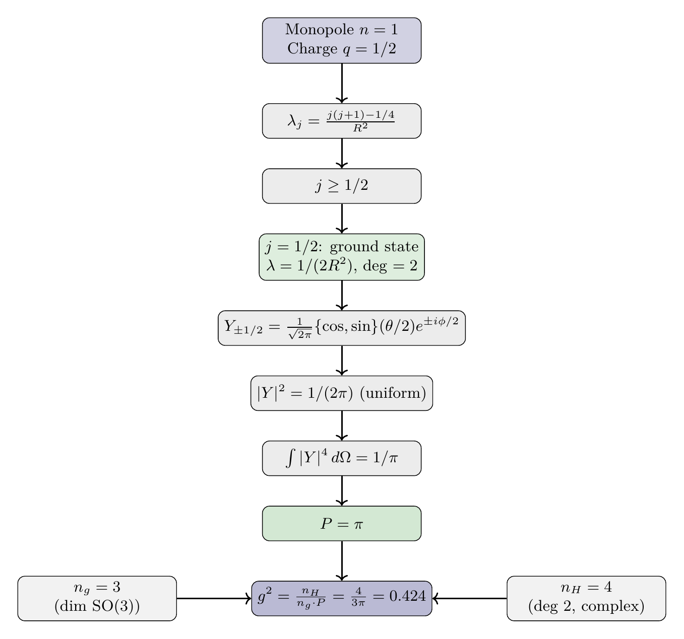
Connection to Coupling: \(g^2 = 4/(3\pi)\)
Every factor in the gauge coupling formula traces to the monopole harmonic results:
where:
- \(n_H = 4\): Higgs degrees of freedom—complex doublet = 4 real d.o.f. (from \(j = 1/2\), degeneracy 2, complex)
- \(n_g = 3\): Gauge generators—\(\dim(\text{SO}(3)) = 3\) from \(S^2\) isometry (Chapter 9)
- \(P = \pi\): Participation ratio from this chapter (Theorem thm:P2-Ch11-participation-ratio)
Comparison with experiment: \(g^2_{\mathrm{exp}} \approx 0.426\). Agreement: \(\mathbf{99.5\%}\).
The coupling formula has the physical structure:
This is the natural form for a coupling: sources in numerator, geometric dilution in denominator.
Polar field form of \(g^2\): In the polar variable \(u = \cos\theta\), the coupling is computed directly as:
Chapter Summary
This chapter derived the monopole harmonics on \(S^2\)—the eigenfunctions of the covariant Laplacian in the Dirac monopole background. The key results:
- Eigenvalue spectrum: \(\lambda_j = [j(j+1) - q^2]/R^2\) with \(j \geq |q|\).
- Ground state (\(q = 1/2\)): \(j = 1/2\), \(\lambda = 1/(2R^2)\), degeneracy 2, forming an SU(2) doublet (the Higgs).
- Explicit harmonics: \(Y_{\pm 1/2} = \frac{1}{\sqrt{2\pi}}\{\cos,\sin\}(\theta/2)\,e^{\pm i\phi/2}\).
- Uniformity: \(|Y|^2 = 1/(2\pi)\) is constant over \(S^2\) (from the Pythagorean identity).
- Fourth moment: \(\int |Y|^4\, d\Omega = 1/\pi\) (from uniformity).
- Participation ratio: \(P = \pi\) (from fourth moment).
- Gauge coupling: \(g^2 = n_H/(n_g \cdot P) = 4/(3\pi) \approx 0.424\), matching experiment to 99.5%.
Polar field perspective: In the variable \(u = \cos\theta\), the monopole harmonic densities become linear: \(|Y_\pm|^2 = (1\pm u)/(4\pi)\). Uniformity reduces to \((1+u)+(1-u) = 2\). The coupling integral collapses to \(\int_{-1}^{+1}(1+u)^2\,du = 8/3\), with the factor \(3 = 1/\langle u^2\rangle\) traced to the second moment of \(\cos\theta\) on \(S^2\).
Every factor traces to topology, representation theory, or the Pythagorean identity.
Looking ahead: Chapter 12 develops the dimensional reduction framework, showing how KK fails for \(q = 0\) fields versus the interface mechanism for \(q \neq 0\) fields. Chapter 13 derives the modulus stabilization and the 81 \(\mu\)m compact scale.
Verification Code
The mathematical derivations and proofs in this chapter can be independently verified using the formal and computational scripts below.
All verification code is open source. See the complete verification index for all chapters.