Chapter 119

Philosophical Foundations of TD

Introduction

Parts I–X developed TMT's physical predictions—gauge couplings, particle masses, cosmological parameters, and experimental tests. This chapter opens a new line of investigation: what does TMT's geometric structure tell us about the nature of prediction itself?

The Temporal Determination Framework (TDF) is a theory of probabilistic prediction built on TMT's geometry. Its central insight is that the future is ontically determined by the initial S$^2$ configurations of all particles, but epistemically probabilistic because these configurations are inaccessible. This resolves the tension between determinism and quantum probability by localizing randomness to epistemic access rather than to ontology.

Scaffolding Interpretation

In TMT, the $S^2$ provides mathematical scaffolding whose physical consequence is the pattern of quantum numbers, gauge couplings, and internal states. TDF extends this: the $S^2$ configurations also serve as hidden variables that determine individual outcomes while remaining inaccessible to measurement. All physical predictions remain 4D observables.

What Is Temporal Determination?

The Central Question

The prediction problem asks: given TMT's geometric structure, what statements about the future can be made with mathematical certainty, and what remains fundamentally uncertain?

Three historical answers frame the discussion:

Classical (Laplace): An omniscient intellect knowing all positions and momenta could compute the entire future. The universe is a clockwork.

Quantum (Copenhagen): Fundamental randomness exists. The future is intrinsically indeterminate until observation collapses the wavefunction. No hidden variables exist (Bell's theorem).

TMT (This chapter): The future IS determined by hidden variables ($S^2$ configurations), but these are epistemically inaccessible. Probability is real but not fundamental—it reflects geometric ignorance. Aggregate futures are computable from geometry alone.

The TMT Resolution of the Determinism Debate

Part 7 (\S57.3) establishes the principle: classical mechanics is deterministic, and QM emerges from classical mechanics on $S^2$. The underlying physics is therefore deterministic but unpredictable, due to unknown initial conditions on $S^2$, chaotic dynamics on the energy shell, and the fact that $S^2$ degrees of freedom are hidden variables. This resembles de Broglie-Bohm theory, with $S^2$ providing the hidden variables.

The critical insight is that TMT resolves the tension between determinism and quantum probability not by denying either, but by localizing randomness to epistemic access rather than to ontology.

Indeterminacy vs Determinism

Ontic and Epistemic States

Definition 119.8 (Ontic State)

The ontic state $\omega$ of a physical system is the complete specification of all physical degrees of freedom, including the $S^2$ configuration for each particle:

$$ \omega = \{(x_i^\mu,\,\Omega_i) : i = 1,\ldots,N\} $$ (119.1)

where $x_i^\mu$ is the 4D spacetime position and $\Omega_i = (\theta_i,\phi_i)\in S^2$ is the $S^2$ configuration.

Definition 119.9 (Epistemic State)

The epistemic state $\varepsilon$ is a probability distribution over ontic states, reflecting an observer's knowledge:

$$ \varepsilon = \mu(\omega) $$ (119.2)

where $\mu$ is a measure on the space of ontic states.

Theorem 119.1 (Ontic-Epistemic Distinction in TMT)

In TMT: (1) The ontic state is always well-defined (determinism holds). (2) The $S^2$ components of the ontic state are epistemically inaccessible. (3) The epistemic state has a unique natural form (the microcanonical measure). (4) Quantum probability IS the natural epistemic distribution.

Proof.

Step 1: From P1 ($ds_6^{\,2} = 0$), particles follow deterministic null geodesics in the 6D scaffolding space $\mathcal{M}^4\times S^2$. The ontic state evolves deterministically.

Step 2: The $S^2$ coordinates are not directly observable—they manifest only through projections to 4D (via gauge charges, spin states, etc.). No measurement can determine the precise $(\theta,\phi)$ location on $S^2$.

Step 3: From Part 7 (Theorem 52.2), the microcanonical distribution on $S^2$ is uniform:

$$ \rho_{\text{classical}}(\theta,\phi) = \frac{1}{4\pi} $$ (119.3)

This is the unique distribution that maximizes entropy, is invariant under SO(3) rotations, and equals the quantum probability (Part 7 Theorem 53.3).

Step 4: Part 7 Theorem 53.3 proves:

$$ \rho_{\text{classical}} = |Y_+|^2 + |Y_-|^2 = \frac{1}{4\pi} $$ (119.4)

The classical microcanonical distribution equals the quantum ground state probability. Quantum probability IS epistemic uncertainty about $S^2$ configurations.

(See: Part 7 \S\S52–53,57; Part 12 Ch 140) □

The Ensemble Interpretation Extended

Part 7 establishes the ensemble interpretation for quantum mechanics: the “wavefunction” is an ensemble distribution, “measurement” is sampling from the ensemble, and “collapse” is updating knowledge after sampling. The measurement problem dissolves—there was never superposition of individual states, only ensemble distributions.

Theorem 119.2 (Extension to Macroscopic Systems)

The ensemble interpretation extends to macroscopic systems and future predictions: (1) The “future state” is an ensemble over possible configurations. (2) “Observation of the future” is sampling from this ensemble. (3) “What actually happens” is one sample from the distribution.

Proof.

The ensemble interpretation depends only on: deterministic underlying dynamics (true for any particle count), inaccessible hidden variables (the $S^2$ configurations remain hidden regardless of system size), and a natural measure on hidden variables (the microcanonical measure is defined for any $N$). None of these depend on particle number.

(See: Part 7 \S57.3; Part 12 Ch 140) □

The Framework

The Arrow of Time

The arrow of time—the observed asymmetry between past and future— arises from a boundary condition: the initial state $\Sigma_0$ was a state of very low entropy (highly constrained $S^2$ configurations).

Theorem 119.3 (Deterministic Evolution)

There exists a unique evolution operator $\Phi_t:\mathcal{F}_0\to\mathcal{F}_t$ such that:

$$ \Sigma_t = \Phi_t(\Sigma_0) $$ (119.5)

The entire future of the universe is determined by $\Sigma_0$.

Proof.

Step 1: From P1, all particles follow null geodesics in the 6D scaffolding:

$$ ds_6^{\,2} = g_{\mu\nu}dx^\mu dx^\nu + R_0^2\,d\Omega^2 = 0 $$ (119.6)

Step 2: Null geodesic equations are second-order ODEs with unique solutions given initial conditions $(x^\mu(0),\dot{x}^\mu(0),\Omega(0),\dot{\Omega}(0))$.

Step 3: Conservation laws (Part 6A Ch. 41) provide deterministic constraints: $\nabla_A T^{AB} = 0$.

Step 4: Therefore $\Phi_t$ exists and is unique.

(See: Part 6A Ch 41; Part 12 Ch 140) □

Theorem 119.4 (Epistemic Inaccessibility of Initial Conditions)

The initial ontic state $\Sigma_0$ is epistemically inaccessible because: (1) $S^2$ configurations are never directly measured. (2) The Big Bang occurred before any observer existed. (3) Chaotic dynamics amplify small uncertainties exponentially: $|\delta\Omega(t)|\sim|\delta\Omega(0)|e^{\lambda t}$ where $\lambda > 0$ is the Lyapunov exponent.

Proof.

(1) From the scaffolding interpretation, $S^2$ is not a physical space one can probe. Measurements yield 4D projections, not $S^2$ coordinates.

(2) Thermalization in the early universe erases structural information; cosmic horizons and quantum measurement limits prevent recovery.

(3) Part 7 proves that motion on $S^2$ is ergodic (Theorem 52.4). Ergodic systems exhibit exponential sensitivity to initial conditions.

(See: Part 7 Thm 52.4; Part 12 Ch 140) □

Theorem 119.5 (Entropy Increase from S$^2$ Spreading)

If the initial $S^2$ configurations were highly correlated (low entropy), then evolution toward the microcanonical (uniform) distribution represents entropy increase:

$$ S(t) = -\int_{\mathcal{F}_t}\mu_t(\omega)\log\mu_t(\omega)\,d\omega $$ (119.7)

increases toward the maximum value $S_{\text{MC}} = \log(4\pi)$ per particle.

Proof.

Step 1: The microcanonical distribution $\mu_{\text{MC}} = 1/(4\pi)$ maximizes entropy on $S^2$: $S_{\text{MC}} = \log(4\pi)$.

Step 2: Any other distribution $\mu\neq\mu_{\text{MC}}$ satisfies $S[\mu] < S[\mu_{\text{MC}}]$ by the Gibbs inequality.

Step 3: Ergodic dynamics (Part 7 Theorem 52.4) implies $\lim_{t\to\infty}\mu_t = \mu_{\text{MC}}$ for generic initial distributions.

Step 4: Therefore entropy increases from $S[\mu_0]$ toward $\log(4\pi)$. This is the second law of thermodynamics derived from $S^2$ geometry.

(See: Part 7 Thms 52.2,52.4; Part 12 Ch 140) □

The Temporal Determination Principle

Theorem 119.6 (Geometric Origin of Probability)

The probability distribution over future states is not empirical—it follows from P1:

$$ ds_6^{\,2} = 0\quad\Rightarrow\quad\rho_{S^2} = \frac{1}{4\pi} $$ (119.8)

Proof.

The derivation chain is: (1) P1 $\Rightarrow$ particles move on null geodesics in $\mathcal{M}^4\times S^2$. (2) Null geodesics $\Rightarrow$ classical dynamics on $S^2$ with monopole. (3) Classical dynamics $\Rightarrow$ ergodic flow on energy shell. (4) Ergodic flow $\Rightarrow$ microcanonical distribution is the unique equilibrium. (5) Microcanonical distribution $= 1/(4\pi)$ uniform on $S^2$.

Every step is derived, not assumed. The probability distribution is a theorem, not a model.

(See: Part 7 Thms 52.2–52.4,53.3; Part 12 Ch 140) □

The Temporal Determination Principle states: the future is determined but not determinable. More precisely: (1) there exists a unique future $\Sigma_t = \Phi_t(\Sigma_0)$ (ontic determination); (2) we cannot know $\Sigma_0$, hence cannot compute $\Sigma_t$ exactly (epistemic indeterminability); (3) the probability distribution $P(\Sigma_t)$ IS computable from geometry (probabilistic determinability); (4) in the large-$N$ limit, aggregate observables become deterministic (aggregate determination).

This distinguishes TDF from all statistical prediction methods, which rely on empirical regularities that could change. TDF distributions follow from the geometry of $ds_6^{\,2} = 0$ alone and require no historical data, parameter estimation, model selection, or Bayesian priors.

Polar Field Form of TDF Probability

The geometric origin of probability becomes maximally transparent in the polar field variable $u = \cos\theta$. The key property is that the $S^2$ integration measure becomes flat:

$$ d\Omega = \sin\theta\,d\theta\,d\phi \;=\; du\,d\phi $$ (119.9)

so the microcanonical distribution $\rho = 1/(4\pi)$ is a constant function on the flat polar rectangle $[-1,+1]\times[0,2\pi)$ with no Jacobian factors.

In spherical coordinates, the uniformity of $\rho = 1/(4\pi)$ is not visually obvious because the measure $\sin\theta\,d\theta\,d\phi$ carries an angular factor that must cancel against the density. In polar coordinates, both the measure and the density are manifestly flat:

$$ \int_{S^2}\rho\,d\Omega \;=\; \int_0^{2\pi}d\phi\int_{-1}^{+1}\frac{1}{4\pi}\,du \;=\; \frac{1}{4\pi}\cdot 2\pi\cdot 2 \;=\; 1 $$ (119.10)

Every step is polynomial—no trigonometric substitutions needed.

The entropy of the $S^2$ distribution (Theorem thm:P12-Ch86-entropy-increase) likewise simplifies in polar form:

$$ S = -\int_{-1}^{+1}\int_0^{2\pi}\rho(u,\phi)\, \ln\bigl[\rho(u,\phi)\bigr]\,du\,d\phi $$ (119.11)

For the microcanonical $\rho = 1/(4\pi)$:

$$ S_{\mathrm{MC}} = -\frac{1}{4\pi}\ln\!\left(\frac{1}{4\pi}\right) \cdot\underbrace{\int_0^{2\pi}d\phi}_{2\pi} \cdot\underbrace{\int_{-1}^{+1}du}_{2} = \ln(4\pi) $$ (119.12)

The maximum entropy is literally the logarithm of the rectangle area $4\pi$ in flat measure.

For the concentration of measure bound (Theorem thm:P12-Ch86-concentration), the $N$-particle product measure takes the manifestly flat form:

$$ d\mu_N = \prod_{i=1}^{N}\frac{du_i\,d\phi_i}{4\pi} $$ (119.13)

Each factor is uniform on a flat rectangle—the concentration bound follows directly from the product structure with no curvature corrections.

Property	Spherical $(\theta, \phi)$	Polar $(u, \phi)$
Measure	$\sin\theta\,d\theta\,d\phi$	$du\,d\phi$ (flat)
Microcanonical $\rho$	$1/(4\pi)$	$1/(4\pi)$
Normalization check	requires $\int\sin\theta\,d\theta$	trivial: $2\times 2\pi$
Maximum entropy	$\ln(4\pi)$	$\ln(\text{rectangle area})$
Product measure	$\prod_i\sin\theta_i\,d\theta_i\,d\phi_i/(4\pi)$	$\prod_i du_i\,d\phi_i/(4\pi)$
Factorization	hidden by $\sin\theta$	manifest AROUND $\times$ THROUGH

The polar form reveals why the microcanonical distribution is the unique natural measure on $S^2$: it is the only distribution that is constant on the flat rectangle. Any other density would single out preferred values of $u$ (THROUGH direction) or $\phi$ (AROUND direction), breaking the democracy of directions that P1 guarantees.

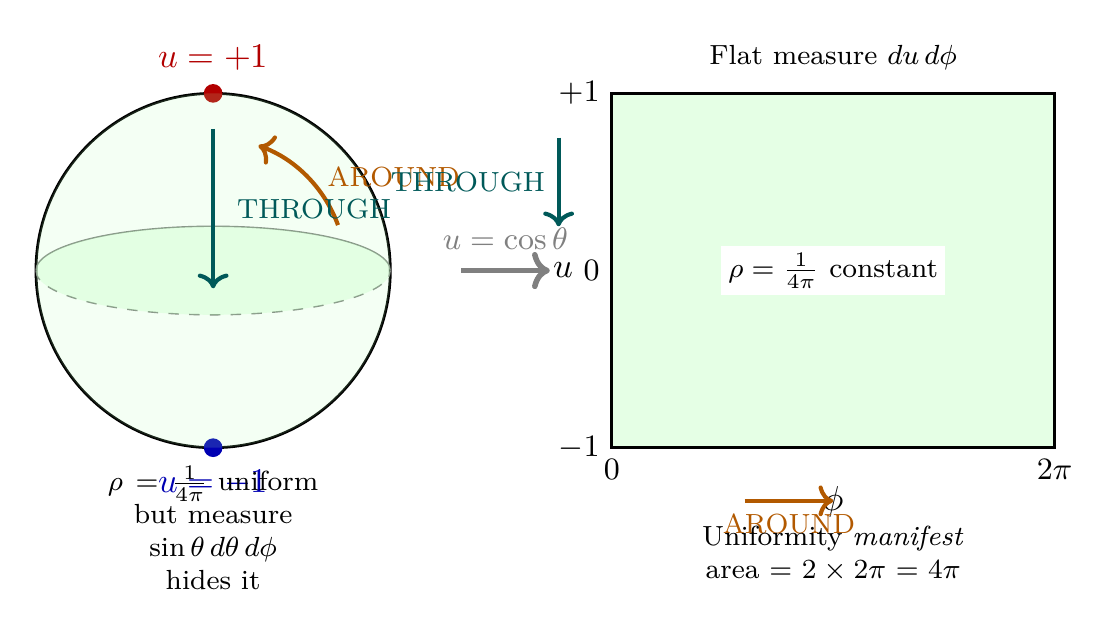
**Figure 119.1:** The microcanonical distribution $\rho = 1/(4\pi)$ on $S^2$. **Left:** On the sphere, uniformity is not visually obvious because the measure $\sin\theta\,d\theta\,d\phi$ carries a latitude-dependent factor. **Right:** In polar field coordinates, the flat measure $du\,d\phi$ makes uniformity manifest—the density is constant on the rectangle with area $4\pi$. This is why the microcanonical distribution is the unique natural measure: it is the only constant function on the flat rectangle.

Scaffolding Interpretation

Scaffolding note: The polar field variable $u = \cos\theta$ is a coordinate choice, not a new physical assumption. The microcanonical distribution $\rho = 1/(4\pi)$ is the same in both coordinate systems; the polar form simply makes its uniformity and entropy properties manifest by removing the $\sin\theta$ Jacobian from the integration measure.

Concentration of Measure and Aggregate Certainty

Theorem 119.7 (Concentration of Measure on S$^2$)

For $N$ particles, each with $S^2$ coordinate $\Omega_i$ distributed uniformly on $S^2$, let $A(\Omega_1,\ldots,\Omega_N)$ be an aggregate observable with Lipschitz constant $L$. Then:

$$ P\bigl(|A-\langle A\rangle|>\varepsilon\bigr) \leq 2\exp\!\left(-\frac{N\varepsilon^2}{2L^2}\right) $$ (119.14)

Proof.

This is Lévy's lemma applied to the product measure on $(S^2)^N$. The uniform measure on $S^2$ is the normalized area measure $d\mu = (1/(4\pi))\sin\theta\,d\theta\,d\phi$. The product measure on $(S^2)^N$ is $d\mu_N = \prod_i d\mu_i$. Lévy's lemma states that for product measures on high-dimensional spheres, Lipschitz functions concentrate around their mean with exponential tails. The bound follows from the isoperimetric inequality on $S^2$.

(See: Part 12 Ch 140) □

As $N\to\infty$, aggregate observables become deterministic: $\lim_{N\to\infty}P(|A-\langle A\rangle|>\varepsilon) = 0$ for any fixed $\varepsilon > 0$. The minimum number of particles required to achieve probability $1-\delta$ that $|A-\langle A\rangle| <\varepsilon$ is:

$$ N_{\min} = \frac{2L^2}{\varepsilon^2}\ln\frac{2}{\delta} $$ (119.15)

For $\varepsilon = 0.01$ (1% accuracy), $\delta = 0.01$ (99% confidence), and $L = 1$: $N_{\min}\approx 106{,}000$. Systems with $N > 10^5$ particles have aggregate properties predictable to 1% with 99% confidence.

Philosophical Status

Predictability and Limits

TDF-predictable quantities require: (1) aggregate dependence (collective, not individual properties); (2) $N\gg N_{\min}$ particles; (3) bounded Lipschitz constant; (4) $S^2$ equilibrium reached. Examples include thermodynamic properties, equilibrium statistical distributions, large-scale cosmological parameters, and ensemble averages.

TDF-unpredictable quantities include individual measurement outcomes, precise timing of chaotic events, small-$N$ fluctuations, and non-equilibrium transients.

The “Mule Problem”

A critical fluctuation is a small-$N$ event (unpredictable by TDF) that triggers large-scale consequences through amplification mechanisms. TDF predictions can fail when $\partial A_{\text{aggregate}}/\partial A_{\text{individual}}\to\infty$, i.e., when individual events have unbounded influence on aggregates. This is a fundamental limit, not a failure of TDF—it correctly identifies where prediction becomes impossible.

Relation to Interpretations of Quantum Mechanics

TDF is most closely aligned with de Broglie-Bohm (pilot wave) theory, with $S^2$ providing the hidden variables. Unlike Bohm, TDF derives the hidden variable structure from geometry rather than postulating it.

Table 119.1: TDF relation to QM interpretations

Interpretation	Ontic State?	Hidden Variables?	TDF Compatible?
Copenhagen	Undefined	No	Partial
Many-Worlds	Yes (branching)	No	No
de Broglie-Bohm	Yes (deterministic)	Yes	Yes
QBism	No (epistemic only)	No	Partial
TMT/TDF	Yes ($S^2$ configs)	Yes ($S^2$)	Definition

In TDF, “superposition” is a feature of the epistemic state, not the ontic state. Each individual system has a definite $S^2$ configuration. “Collapse” is Bayesian updating upon receiving new information. No physical process corresponds to collapse.

Chapter Summary

Key Result

Philosophical Foundations of Temporal Determination

TDF resolves the determinism–probability tension: the future is ontically determined by $S^2$ configurations but epistemically probabilistic because these configurations are inaccessible. The probability distribution $\rho = 1/(4\pi)$ is a geometric theorem from P1, not an empirical assumption. Concentration of measure implies that aggregate observables become deterministic for $N\gg N_{\min}$, where $N_{\min} = 2L^2\varepsilon^{-2}\ln(2/\delta)$. In the polar field variable $u = \cos\theta$, the flat measure $du\,d\phi$ makes uniformity of $\rho$ manifest: the microcanonical distribution is the unique constant function on the polar rectangle $[-1,+1]\times[0,2\pi)$, and the maximum entropy $\ln(4\pi)$ equals the logarithm of the rectangle area.

Table 119.2: Chapter 86 results summary

Result	Value	Status	Reference
Ontic-epistemic distinction	$S^2$ hidden variables	PROVEN	Thm thm:P12-Ch86-ontic-epistemic
Deterministic evolution	$\Sigma_t = \Phi_t(\Sigma_0)$	PROVEN	Thm thm:P12-Ch86-deterministic-evolution
Geometric probability	$\rho = 1/(4\pi)$	PROVEN	Thm thm:P12-Ch86-geometric-probability
Concentration of measure	$P\leq 2e^{-N\varepsilon^2/2L^2}$	PROVEN	Thm thm:P12-Ch86-concentration
Entropy increase	$S\to\log(4\pi)$	PROVEN	Thm thm:P12-Ch86-entropy-increase

Verification Code

The mathematical derivations and proofs in this chapter can be independently verified using the formal and computational scripts below.

◆ Lean 4 Formal proof verification Coming Soon ● Python Numerical verification & plots Coming Soon ★ Mathematica Symbolic computation & CAS verification Coming Soon

All verification code is open source. See the complete verification index for all chapters.

Property	Spherical \((\theta, \phi)\)	Polar \((u, \phi)\)
Measure	\(\sin\theta\,d\theta\,d\phi\)	\(du\,d\phi\) (flat)
Microcanonical \(\rho\)	\(1/(4\pi)\)	\(1/(4\pi)\)
Normalization check	requires \(\int\sin\theta\,d\theta\)	trivial: \(2\times 2\pi\)
Maximum entropy	\(\ln(4\pi)\)	\(\ln(\text{rectangle area})\)
Product measure	\(\prod_i\sin\theta_i\,d\theta_i\,d\phi_i/(4\pi)\)	\(\prod_i du_i\,d\phi_i/(4\pi)\)
Factorization	hidden by \(\sin\theta\)	manifest AROUND \(\times\) THROUGH

Result	Value	Status	Reference
Ontic-epistemic distinction	\(S^2\) hidden variables	PROVEN	Thm thm:P12-Ch86-ontic-epistemic
Deterministic evolution	\(\Sigma_t = \Phi_t(\Sigma_0)\)	PROVEN	Thm thm:P12-Ch86-deterministic-evolution
Geometric probability	\(\rho = 1/(4\pi)\)	PROVEN	Thm thm:P12-Ch86-geometric-probability
Concentration of measure	\(P\leq 2e^{-N\varepsilon^2/2L^2}\)	PROVEN	Thm thm:P12-Ch86-concentration
Entropy increase	\(S\to\log(4\pi)\)	PROVEN	Thm thm:P12-Ch86-entropy-increase