Chapter 96

Berry Phase and Spinors

\usepackage{tikz}

Introduction

Spinor structure—the property that a wavefunction acquires a sign flip $\psi\to -\psi$ under $2\pi$ rotation—is normally postulated as a fundamental feature of quantum mechanics. In the Standard Model, fermions are spinors because they sit in half-integer representations of the Lorentz group, and this property is taken as axiomatic.

TMT derives spinor structure from geometry. On the $S^2$ scaffolding endowed with its topologically required monopole ($qg_m = 1/2$ from the Dirac quantization condition), any charged particle transported around a closed path acquires a Berry phase proportional to the enclosed solid angle. For a great-circle path ($\Omega = 2\pi$), the Berry phase is exactly $\pi$, producing $\psi\to e^{i\pi}\psi = -\psi$—the defining spinor sign flip. No quantum postulate is needed; the result is purely geometric and topological.

This chapter derives the Berry phase on $S^2$ in full detail, demonstrates the emergence of spinor structure, and shows how this connects to the Higgs doublet's transformation properties and to the physical interpretation of spin as a circulation direction.

The Geometric Phase

Berry Phase in General

The Berry phase (also called the geometric phase) is the phase acquired by a quantum or classical system when it is adiabatically transported around a closed loop in parameter space. For a charged particle in a magnetic field, the Berry phase equals the magnetic flux enclosed by the path:

$$ \gamma = q\oint_C \mathbf{A}\cdot d\mathbf{l} = q\,\Phi_B $$ (96.1)

where $q$ is the charge, $\mathbf{A}$ is the gauge potential, and $\Phi_B$ is the magnetic flux through any surface bounded by the closed curve $C$.

The Berry phase is geometric: it depends only on the path geometry (specifically, the enclosed flux or solid angle), not on the speed of traversal or other dynamical details. This geometric character is crucial for TMT, because it means the Berry phase is determined entirely by the $S^2$ topology.

The Monopole Gauge Field on $S^2$

The topologically required monopole on $S^2$ (established in Part 3 from $\pi_2(S^2)=\mathbb{Z}$) generates a gauge field. In the standard northern-patch coordinates $(\theta,\phi)$ on $S^2$, the gauge potential for the minimal monopole ($g_m = 1/2$) is:

$$ A_\phi = g_m(1-\cos\theta) = \tfrac{1}{2}(1-\cos\theta) $$ (96.2)

with $A_\theta = 0$. The corresponding magnetic field is radially directed and satisfies:

$$ \oint_{S^2} \mathbf{B}\cdot d\mathbf{S} = 4\pi g_m = 2\pi $$ (96.3)

which is the total magnetic flux through $S^2$.

Convention: $q=1$, $g_m=1/2$

TMT uses the standard Dirac quantization convention:

$$ qg_m = \tfrac{1}{2} $$ (96.4)

with $q=1$ and $g_m = 1/2$. This is equivalent to the Wu–Yang convention ($q=1/2$, $g_m=1$) since only the product $qg_m$ enters physical observables. Both conventions give the same Berry phase.

Theorem 96.1 (Berry Phase on $S^2$)

A particle with charge $q=1$ transported around a closed path on $S^2$ enclosing solid angle $\Omega$ acquires the Berry phase:

$$ \boxed{\gamma = qg_m\times\Omega = \frac{\Omega}{2}} $$ (96.5)

Proof.

Step 1: Consider a circular path at constant colatitude $\theta_0$ on $S^2$. The Berry phase is the line integral of the gauge potential around this path:

$$ \gamma = q\oint A_\phi\,d\phi = q\int_0^{2\pi}g_m(1-\cos\theta_0)\,d\phi $$ (96.6)

Step 2: Evaluating the integral with $q=1$, $g_m=1/2$:

$$\begin{aligned} \gamma &= 1\times\tfrac{1}{2}(1-\cos\theta_0)\times 2\pi \\ &= \pi(1-\cos\theta_0) \end{aligned}$$ (96.28)

Step 3: The solid angle enclosed by the path (the spherical cap from the north pole down to colatitude $\theta_0$) is:

$$ \Omega = \int_0^{2\pi}d\phi\int_0^{\theta_0}\sin\theta\,d\theta = 2\pi(1-\cos\theta_0) $$ (96.7)

Step 4: Comparing Eqs. (eq:ch63-berry-eval) and (eq:ch63-solid-angle):

$$ \gamma = \frac{\Omega}{2} = qg_m\times\Omega $$ (96.8)

This holds for any circular path. By deformation invariance of the Berry phase (gauge invariance), it extends to arbitrary closed paths enclosing solid angle $\Omega$.

(See: Part 3 §8 (Dirac quantization), Part 7A §54.1) □

Polar Field Form of the Berry Phase

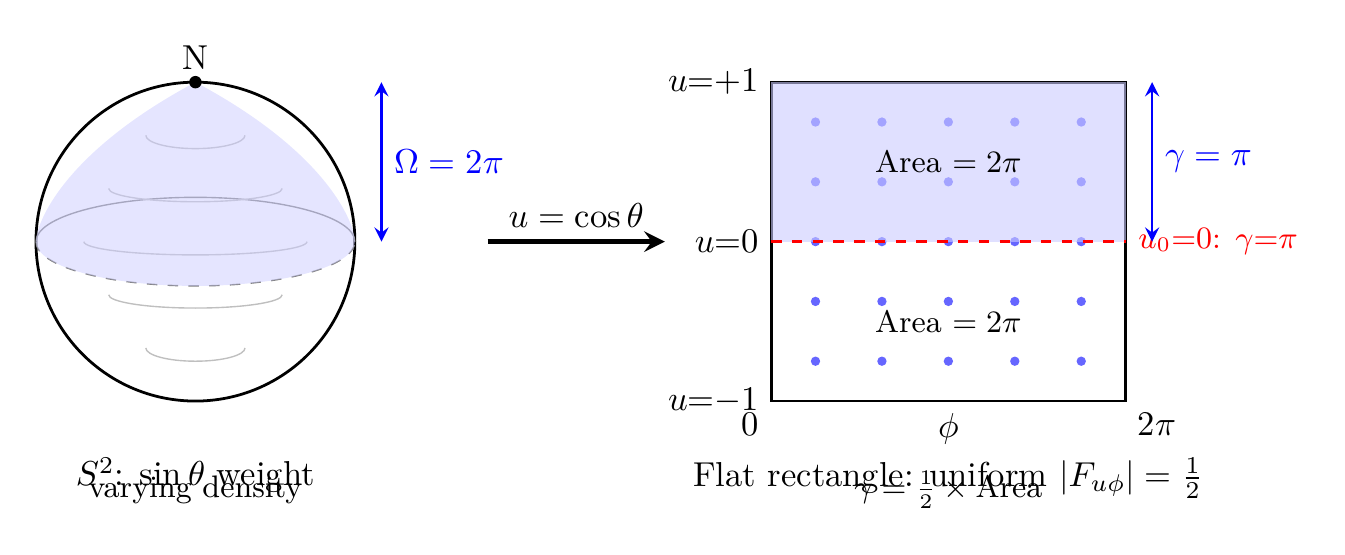
In polar field coordinates $u = \cos\theta$, $\phi\in[0,2\pi)$, the Berry phase becomes strikingly transparent. Since $\cos\theta_0 = u_0$, the solid angle of a polar cap down to colatitude $\theta_0$ is:

$$ \Omega = 2\pi(1-\cos\theta_0) = 2\pi(1-u_0) $$ (96.9)

and the Berry phase is:

$$ \boxed{\gamma = \frac{\Omega}{2} = \pi(1-u_0)} $$ (96.10)

This is linear in $u_0$. The Berry phase is simply proportional to the “distance from the north pole” measured in the polar coordinate.

The gauge potential in polar coordinates reads:

$$ A_\phi = \tfrac{1}{2}(1-u), \qquad A_u = 0 $$ (96.11)

and the field strength is the constant:

$$ F_{u\phi} = \partial_u A_\phi - \partial_\phi A_u = -\tfrac{1}{2} $$ (96.12)

The magnitude $|F_{u\phi}| = 1/2$ is constant everywhere on $S^2$—the monopole flux is uniformly distributed on the flat polar rectangle $[-1,+1]\times[0,2\pi)$.

Scaffolding Interpretation

The linear Berry phase $\gamma = \pi(1-u_0)$ is a scaffolding result: the physical content is $\gamma = \Omega/2$, and polar coordinates merely make the underlying uniformity manifest. Per Part A (Interpretive Framework), the flat-rectangle picture is a calculational tool, not a claim about physical geometry.

Table 96.1: Berry phase: standard vs. polar field coordinates

Quantity	Standard $(\theta,\phi)$	Polar $(u,\phi)$
Gauge potential	$A_\phi = \frac{1}{2}(1-\cos\theta)$	$A_\phi = \frac{1}{2}(1-u)$
Field strength	varies with $\sin\theta$ factor	$F_{u\phi} = -\frac{1}{2}$ (constant)
Solid angle	$2\pi(1-\cos\theta_0)$	$2\pi(1-u_0)$
Berry phase	$\pi(1-\cos\theta_0)$	$\pi(1-u_0)$ (linear)
Spinor case	$\theta_0 = \pi/2$, $\gamma = \pi$	$u_0 = 0$, $\gamma = \pi$

**Figure 96.1:** Berry phase on $S^2$ and the flat polar rectangle. **Left:** The monopole distributes flux non-uniformly in $(\theta,\phi)$ coordinates due to the $\sin\theta$ measure. **Right:** In polar field coordinates $(u,\phi)$, the flux density $|F_{u\phi}| = 1/2$ is constant. The Berry phase for a polar cap to $u_0$ equals half the enclosed rectangle area. The equator ($u_0 = 0$, red dashed) gives $\gamma = \pi$—the spinor sign flip.

Key Special Cases

Table 96.2: Berry phase for special paths on $S^2$

Path	$\theta_0$	Solid Angle $\Omega$	Berry Phase $\gamma$
Infinitesimal loop	$\epsilon\to 0$	$\sim\pi\epsilon^2$	$\sim\pi\epsilon^2/2$
Polar cap ($60^\circ$)	$\pi/3$	$\pi$	$\pi/2$
Great circle (equator)	$\pi/2$	$2\pi$	$\boldsymbol{\pi}$
$120^\circ$ cap	$2\pi/3$	$3\pi$	$3\pi/2$
Full hemisphere	$\pi$	$4\pi$	$2\pi$

The critical entry is the great circle: $\gamma = \pi$. This is exactly the phase that produces the spinor sign flip.

Adiabatic Evolution on $S^2$

Adiabatic Transport and the Monopole Connection

The Berry phase arises from the connection on the principal $U(1)$ bundle over $S^2$ defined by the monopole field. In the language of differential geometry, the gauge potential $A_\phi = g_m(1-\cos\theta)$ defines a connection 1-form on this bundle, and the Berry phase is the holonomy of this connection around the closed loop.

For adiabatic transport—where the system evolves slowly compared to internal timescales—the Berry phase is the only phase acquired beyond the dynamical phase. The adiabatic condition is satisfied whenever the orbital period on $S^2$ is much shorter than the timescale of parameter changes. In TMT, the natural orbital frequency is $\omega_0 = \pi c/L_\xi \approx1.16e13\,rad/s$ (from Chapter 61), so adiabaticity is ensured for all macroscopic processes.

Path Independence and Topology

The Berry phase depends only on the solid angle enclosed by the path, not on the detailed shape of the path. Two paths enclosing the same solid angle give the same Berry phase. This is a direct consequence of gauge invariance: the Berry phase equals the flux through the enclosed surface, and the monopole flux is distributed uniformly over $S^2$.

More precisely, for the monopole with $g_m = 1/2$, the magnetic field is:

$$ B_r = \frac{g_m}{R_0^2} = \frac{1}{2R_0^2} $$ (96.13)

which is uniform in the radial direction (the “Coulomb-like” field on $S^2$). The flux through any region of solid angle $\Omega$ is $\Phi = g_m\,\Omega = \Omega/2$, confirming $\gamma = q\Phi = \Omega/2$.

Polar Field Form: Berry Phase as Rectangle Area

The path-independence of the Berry phase becomes geometrically obvious in polar field coordinates. On the flat rectangle $(u,\phi)\in[-1,+1]\times[0,2\pi)$, the monopole field strength $F_{u\phi} = -1/2$ is constant (Eq. eq:ch63-F-polar). For any closed path enclosing a region $\mathcal{R}$ on the rectangle, the Berry phase is:

$$ \gamma = \int_{\mathcal{R}} |F_{u\phi}|\,du\,d\phi = \frac{1}{2}\,\text{Area}(\mathcal{R}) $$ (96.14)

where $\text{Area}(\mathcal{R})$ is the coordinate area on the flat rectangle. Path independence is now trivial: paths enclosing the same coordinate area give the same Berry phase, because the “flux density” is everywhere the same.

For a polar cap (north pole to latitude $u_0$), the enclosed coordinate area is $2\pi(1-u_0)$, giving:

$$ \gamma = \frac{1}{2}\times 2\pi(1-u_0) = \pi(1-u_0) $$ (96.15)

confirming the result of Eq. (eq:ch63-berry-polar). The total rectangle area is $2\pi\times 2 = 4\pi$, so $\gamma_\text{max} = 2\pi$—a full $2\pi$ phase for the entire sphere, consistent with Eq. (eq:ch63-total-flux).

Scaffolding Interpretation

The “Berry phase = half the rectangle area” identity is a scaffolding restatement of the geometric result $\gamma = \Omega/2$. The flat rectangle is the computational coordinate chart, not physical space. Per Part A (Interpretive Framework), the physical content is the enclosed solid angle.

Non-Contractible Loops

On $S^2$, every closed loop is contractible (since $\pi_1(S^2)=0$). This means the Berry phase is entirely determined by the enclosed solid angle, with no additional topological contribution from winding numbers. However, the Berry phase itself is topologically non-trivial because of the monopole: the total flux $4\pi g_m = 2\pi$ through $S^2$ is quantized and cannot be removed by gauge transformations. This is the content of the Dirac quantization condition $qg_m\in\mathbb{Z}/2$.

Connection to Spinor Structure

The Spinor Sign Flip

The defining property of a spinor is that it changes sign under a $2\pi$ rotation:

$$ \psi \xrightarrow{2\pi\text{ rotation}} -\psi $$ (96.16)

and returns to its original value only after a $4\pi$ rotation. In standard quantum mechanics, this is postulated for half-integer spin particles. In TMT, it is derived.

Theorem 96.2 (Spinor Structure from Berry Phase)

With the Dirac quantization condition $qg_m = 1/2$, a particle transported around a great circle on $S^2$ (enclosing solid angle $\Omega = 2\pi$) acquires phase $\pi$:

$$ \boxed{\psi \xrightarrow{2\pi\text{ orbit}} e^{i\pi}\psi = -\psi} $$ (96.17)

Two complete orbits ($4\pi$ total solid angle) restore the original state:

$$ \psi \xrightarrow{4\pi\text{ orbit}} e^{2i\pi}\psi = +\psi $$ (96.18)

This is the defining property of a spinor. It is derived from $S^2$ geometry with no quantum postulates.

Proof.

Step 1: From Theorem thm:P7-Ch63-berry-phase-S2, the Berry phase for a path enclosing solid angle $\Omega$ is:

$$ \gamma = \frac{\Omega}{2} $$ (96.19)

Step 2: For a great circle ($\Omega = 2\pi$):

$$ \gamma = \frac{2\pi}{2} = \pi $$ (96.20)

Step 3: The wavefunction transforms as:

$$ \psi \to e^{i\gamma}\psi = e^{i\pi}\psi = -\psi $$ (96.21)

Step 4: For two great circles ($\Omega = 4\pi$):

$$ \gamma = \frac{4\pi}{2} = 2\pi \quad\Longrightarrow\quad \psi \to e^{2i\pi}\psi = +\psi $$ (96.22)

Conclusion: The wavefunction has period $4\pi$, not $2\pi$. This is exactly the double-cover property of spinors: $\text{SU}(2)\to\text{SO}(3)$ with kernel $\mathbb{Z}_2$.

(See: Part 7A §54.2, Part 3 §8 (Dirac quantization)) □

Polar Field Form of the Spinor Sign Flip

In polar coordinates, the spinor sign flip acquires a beautifully simple geometric interpretation. A great circle on $S^2$ corresponds to the equator $u = 0$ in the polar chart. A polar cap from the north pole ($u = +1$) to the equator ($u_0 = 0$) encloses:

Coordinate area on the flat rectangle: $\Delta u\times\Delta\phi = 1\times 2\pi = 2\pi$
Berry phase: $\gamma = \pi(1-u_0) = \pi(1-0) = \pi$

The spinor sign flip occurs precisely at the midpoint of the polar rectangle: the equator $u = 0$ bisects the interval $[-1,+1]$, and the Berry phase at this midpoint is exactly $\pi$—half the total phase $2\pi$ accumulated over the entire sphere.

The THROUGH/AROUND decomposition clarifies the structure:

THROUGH ($u$-direction): The Berry phase accumulates linearly as a function of $u_0$: $\gamma = \pi(1-u_0)$. The spinor flip is a THROUGH-direction effect—how far “down” the $u$-axis the path extends.
AROUND ($\phi$-direction): The $2\pi$ azimuthal traversal is the “winding” that closes the path. Without the full $\phi$ circuit, the path is open and the phase is gauge-dependent.

The double-cover ($4\pi$ restoration) in polar language means traversing the entire rectangle twice: area $= 2\times 4\pi = 8\pi$, but modulo $4\pi$ the net area is $4\pi$, and $\gamma = 2\pi \equiv 0$.

Table 96.3: Spinor sign flip: standard vs. polar field coordinates

Feature	Standard $(\theta,\phi)$	Polar $(u,\phi)$
Great circle	$\theta_0 = \pi/2$	$u_0 = 0$ (rectangle midpoint)
Solid angle	$\Omega = 2\pi$	Area $= 2\pi$
Berry phase	$\gamma = \pi$	$\gamma = \pi(1-0) = \pi$
Sign flip	$e^{i\pi} = -1$	Half-rectangle area
$4\pi$ restoration	Two orbits	Full rectangle twice

Scaffolding Interpretation

The “equator = rectangle midpoint” identification is a property of the polar coordinate chart. The physical content is $\gamma = \pi$ for $\Omega = 2\pi$; the flat-rectangle visualization provides intuition but is not itself a physical claim. Per Part A (Interpretive Framework).

No $\hbar$ Required

Corollary 96.4 (Spinor Structure is Classical)

The spinor property $\psi\to -\psi$ under $2\pi$ rotation is entirely geometric. It does not require $\hbar$.

The Berry phase depends on three quantities—the charge $q$ (topologically quantized), the monopole charge $g_m$ (topologically quantized), and the solid angle $\Omega$ (geometric)—none of which involve $\hbar$. The spinor structure of matter is therefore a consequence of $S^2$ topology, not a quantum postulate.

Physical Interpretation of Spin

Theorem 96.3 (Classical Interpretation of Spin)

The two components $Y_+$ and $Y_-$ of the monopole harmonic ground state ($j=1/2$) correspond to opposite circulation directions on $S^2$:

$$ Y_+ \sim e^{+i\phi/2} \quad(\text{counterclockwise}), \qquad Y_- \sim e^{-i\phi/2} \quad(\text{clockwise}) $$ (96.23)

Table 96.4: Physical interpretation of spin components

Component	Phase factor	Circulation	Classical analogue
$Y_+$	$e^{+i\phi/2}$	Counterclockwise	$+L_z$ orbit
$Y_-$	$e^{-i\phi/2}$	Clockwise	$-L_z$ orbit

In TMT's scaffolding picture, “spin up” means the particle's $S^2$ mode corresponds to counterclockwise circulation (as viewed from the north pole), while “spin down” corresponds to clockwise circulation. The spin quantum number is the classical circulation direction on $S^2$.

Scaffolding Interpretation

The circulation on $S^2$ is a mathematical description of the mode structure, not a claim about literal physical rotation. Per Part A (Interpretive Framework), $S^2$ is scaffolding—the physical observable is the discrete spin quantum number $\pm 1/2$, which the scaffolding derives rather than postulates.

Polar Field Form of Spin Components

In polar field coordinates $(u,\phi)$, the THROUGH/AROUND decomposition gives a clean separation of the spin-$1/2$ monopole harmonics. The $j = 1/2$ modes take the form:

$$ Y_\pm(u,\phi) \propto \sqrt{\frac{1\pm u}{4\pi}}\;e^{\pm i\phi/2} $$ (96.24)

where the THROUGH factor $\sqrt{(1\pm u)/(4\pi)}$ is a simple linear function of $u$, and the AROUND factor $e^{\pm i\phi/2}$ encodes the half-integer winding.

The probability densities are:

$$ |Y_+|^2 = \frac{1+u}{4\pi}, \qquad |Y_-|^2 = \frac{1-u}{4\pi} $$ (96.25)

These are linear in $u$: $Y_+$ is concentrated near the north pole ($u = +1$) and $Y_-$ near the south pole ($u = -1$), with each density vanishing at the opposite pole. On the flat polar rectangle, these are simple ramp functions—the simplest possible non-trivial distributions.

The angular momentum operator in polar coordinates is purely AROUND:

$$ L_z = -i\hbar\,\partial_\phi $$ (96.26)

acting on $e^{\pm i\phi/2}$ to give eigenvalues $\pm\hbar/2$. The spin quantum number is thus the AROUND winding number, while the THROUGH profile $\sqrt{(1\pm u)/(4\pi)}$ determines the spatial probability distribution.

Table 96.5: Spin components: standard vs. polar field coordinates

Property	Standard $(\theta,\phi)$	Polar $(u,\phi)$
THROUGH profile	$\sin^{1/2}(\theta/2),\,\cos^{1/2}(\theta/2)$	$\sqrt{(1\pm u)/(4\pi)}$ (linear ramp)
AROUND phase	$e^{\pm i\phi/2}$	$e^{\pm i\phi/2}$ (identical)
$\|Y_\pm\|^2$	Trigonometric	$(1\pm u)/(4\pi)$ (linear)
$L_z$	$-i\hbar\,\partial_\phi$	$-i\hbar\,\partial_\phi$ (pure AROUND)
Normalization	$\int\sin\theta\,d\theta\,d\phi = 1$	$\int du\,d\phi = 1$ (flat measure)

Connection to the Higgs Doublet

Corollary 96.5 (Higgs Spinor Structure)

The Higgs field $H$ is a section of the spin-$1/2$ bundle over $S^2$, defined by the monopole with $qg_m = 1/2$. Its spinor transformation property:

$$ H(\phi + 2\pi) = -H(\phi) $$ (96.27)

is not postulated—it emerges from the monopole Berry phase.

This result connects three apparently independent features of the Standard Model: (1) the Higgs is a doublet under SU(2), (2) fermions are spinors, and (3) the Dirac quantization condition. In TMT, all three trace to the single fact that $\pi_2(S^2)=\mathbb{Z}$ requires a monopole with $qg_m = 1/2$.

The Monopole as the Origin of Quantum Structure

The monopole on $S^2$ provides the topological structure that makes classical mechanics on $S^2$ “look quantum”:

(1) Charge quantization $\to$ discrete spectra. The Dirac quantization condition $qg_m\in\mathbb{Z}/2$ ensures that only discrete values of charge (and correspondingly discrete energy levels) are allowed.

(2) Berry phase $\to$ spinor structure. The half-integer product $qg_m = 1/2$ produces the sign flip $\psi\to -\psi$ under $2\pi$ rotation, which is the defining property of spinors.

(3) Non-trivial bundle $\to$ gauge confinement. The monopole prevents gauge fields from extending to the bulk (Part 6A), forcing the interface mechanism that gives correct gauge couplings.

All three features are consequences of $\pi_2(S^2)=\mathbb{Z}\neq 0$ and the stability/chirality requirement that selects $S^2$ from P1.

Factor Origin Table

Table 96.6: Factor origin table for the spinor Berry phase $\gamma = \pi$

Factor	Value	Origin	Source
$q$	1	Minimal U(1) charge	Dirac quantization, Part 3 §8
$g_m$	$1/2$	Minimal monopole charge	$\pi_2(S^2)=\mathbb{Z}$, Part 3 §8
$qg_m$	$1/2$	Dirac condition	Topological, Part 3 Thm 8.1
$\Omega$	$2\pi$	Solid angle of great circle	Geometry of $S^2$
$\gamma$	$\pi$	$= qg_m\times\Omega = \frac{1}{2}\times 2\pi$	This chapter

Every factor traces to $S^2$ topology and geometry. No free parameters are involved.

Chapter Summary

Key Result

Berry Phase and Spinor Structure

The monopole on $S^2$ (required by $\pi_2(S^2)=\mathbb{Z}$ and the Dirac quantization condition $qg_m = 1/2$) generates a Berry phase $\gamma = \Omega/2$ for any closed path enclosing solid angle $\Omega$. For a great circle ($\Omega = 2\pi$), this gives $\gamma = \pi$, producing the spinor sign flip $\psi\to e^{i\pi}\psi = -\psi$. Spinor structure is therefore derived from $S^2$ geometry—it is not a quantum postulate. The two spin components $Y_\pm$ correspond to opposite circulation directions on $S^2$, and the Higgs doublet's spinor transformation emerges from the same monopole Berry phase.

Polar Field Enhancement. In polar field coordinates $u = \cos\theta$, the Berry phase becomes $\gamma = \pi(1-u_0)$—linear in $u$. The constant field strength $F_{u\phi} = -1/2$ on the flat rectangle $[-1,+1]\times[0,2\pi)$ makes the Berry phase equal to half the enclosed coordinate area. The spinor sign flip occurs at the rectangle midpoint $u_0 = 0$ (the equator), where half the rectangle area gives $\gamma = \pi$. The spin-$1/2$ monopole harmonics have linear probability densities $|Y_\pm|^2 = (1\pm u)/(4\pi)$ on the flat rectangle, with spin quantum number determined by the AROUND winding $e^{\pm i\phi/2}$ and spatial distribution by the THROUGH ramp $\sqrt{(1\pm u)/(4\pi)}$.

Table 96.7: Chapter 63 results summary

Result	Value	Status	Reference
Berry phase on $S^2$	$\gamma = \Omega/2$	PROVEN	Thm thm:P7-Ch63-berry-phase-S2
Spinor from Berry phase	$\psi\to -\psi$ ($2\pi$)	PROVEN	Thm thm:P7-Ch63-spinor-from-berry
Spinor is classical	No $\hbar$ required	PROVEN	Cor cor:P7-Ch63-spinor-classical
Spin = circulation	$Y_\pm\sim e^{\pm i\phi/2}$	PROVEN	Thm thm:P7-Ch63-classical-spin
Higgs is spinor	$H(\phi+2\pi)=-H(\phi)$	PROVEN	Cor cor:P7-Ch63-higgs-spinor

Verification Code

The mathematical derivations and proofs in this chapter can be independently verified using the formal and computational scripts below.

◆ Lean 4 Formal proof verification Coming Soon ● Python Numerical verification & plots Coming Soon ★ Mathematica Symbolic computation & CAS verification Coming Soon

All verification code is open source. See the complete verification index for all chapters.

Quantity	Standard \((\theta,\phi)\)	Polar \((u,\phi)\)
Gauge potential	\(A_\phi = \frac{1}{2}(1-\cos\theta)\)	\(A_\phi = \frac{1}{2}(1-u)\)
Field strength	varies with \(\sin\theta\) factor	\(F_{u\phi} = -\frac{1}{2}\) (constant)
Solid angle	\(2\pi(1-\cos\theta_0)\)	\(2\pi(1-u_0)\)
Berry phase	\(\pi(1-\cos\theta_0)\)	\(\pi(1-u_0)\) (linear)
Spinor case	\(\theta_0 = \pi/2\), \(\gamma = \pi\)	\(u_0 = 0\), \(\gamma = \pi\)

Path	\(\theta_0\)	Solid Angle \(\Omega\)	Berry Phase \(\gamma\)
Infinitesimal loop	\(\epsilon\to 0\)	\(\sim\pi\epsilon^2\)	\(\sim\pi\epsilon^2/2\)
Polar cap (\(60^\circ\))	\(\pi/3\)	\(\pi\)	\(\pi/2\)
Great circle (equator)	\(\pi/2\)	\(2\pi\)	\(\boldsymbol{\pi}\)
\(120^\circ\) cap	\(2\pi/3\)	\(3\pi\)	\(3\pi/2\)
Full hemisphere	\(\pi\)	\(4\pi\)	\(2\pi\)

Feature	Standard \((\theta,\phi)\)	Polar \((u,\phi)\)
Great circle	\(\theta_0 = \pi/2\)	\(u_0 = 0\) (rectangle midpoint)
Solid angle	\(\Omega = 2\pi\)	Area \(= 2\pi\)
Berry phase	\(\gamma = \pi\)	\(\gamma = \pi(1-0) = \pi\)
Sign flip	\(e^{i\pi} = -1\)	Half-rectangle area
\(4\pi\) restoration	Two orbits	Full rectangle twice

Property	Standard \((\theta,\phi)\)	Polar \((u,\phi)\)
THROUGH profile	\(\sin^{1/2}(\theta/2),\,\cos^{1/2}(\theta/2)\)	\(\sqrt{(1\pm u)/(4\pi)}\) (linear ramp)
AROUND phase	\(e^{\pm i\phi/2}\)	\(e^{\pm i\phi/2}\) (identical)
\(\|Y_\pm\|^2\)	Trigonometric	\((1\pm u)/(4\pi)\) (linear)
\(L_z\)	\(-i\hbar\,\partial_\phi\)	\(-i\hbar\,\partial_\phi\) (pure AROUND)
Normalization	\(\int\sin\theta\,d\theta\,d\phi = 1\)	\(\int du\,d\phi = 1\) (flat measure)

Factor	Value	Origin	Source
\(q\)	1	Minimal U(1) charge	Dirac quantization, Part 3 §8
\(g_m\)	\(1/2\)	Minimal monopole charge	\(\pi_2(S^2)=\mathbb{Z}\), Part 3 §8
\(qg_m\)	\(1/2\)	Dirac condition	Topological, Part 3 Thm 8.1
\(\Omega\)	\(2\pi\)	Solid angle of great circle	Geometry of \(S^2\)
\(\gamma\)	\(\pi\)	\(= qg_m\times\Omega = \frac{1}{2}\times 2\pi\)	This chapter

Berry Phase and Spinors

Introduction

The Geometric Phase

Berry Phase in General

The Monopole Gauge Field on \(S^2\)

Convention: \(q=1\), \(g_m=1/2\)

Polar Field Form of the Berry Phase

Key Special Cases

Adiabatic Evolution on \(S^2\)

Adiabatic Transport and the Monopole Connection

Path Independence and Topology

Polar Field Form: Berry Phase as Rectangle Area

Non-Contractible Loops

Connection to Spinor Structure

The Spinor Sign Flip

Polar Field Form of the Spinor Sign Flip

No \(\hbar\) Required

Physical Interpretation of Spin

Polar Field Form of Spin Components

Connection to the Higgs Doublet

The Monopole as the Origin of Quantum Structure

Factor Origin Table

Chapter Summary

Verification Code

Component	Phase factor	Circulation	Classical analogue
\(Y_+\)	\(e^{+i\phi/2}\)	Counterclockwise	\(+L_z\) orbit
\(Y_-\)	\(e^{-i\phi/2}\)	Clockwise	\(-L_z\) orbit

Result	Value	Status	Reference
Berry phase on \(S^2\)	\(\gamma = \Omega/2\)	PROVEN	Thm thm:P7-Ch63-berry-phase-S2
Spinor from Berry phase	\(\psi\to -\psi\) (\(2\pi\))	PROVEN	Thm thm:P7-Ch63-spinor-from-berry
Spinor is classical	No \(\hbar\) required	PROVEN	Cor cor:P7-Ch63-spinor-classical
Spin = circulation	\(Y_\pm\sim e^{\pm i\phi/2}\)	PROVEN	Thm thm:P7-Ch63-classical-spin
Higgs is spinor	\(H(\phi+2\pi)=-H(\phi)\)	PROVEN	Cor cor:P7-Ch63-higgs-spinor