
PBR Theorem and Ontic States
Chapter Overview: This chapter establishes that the \(S^2\) geometric framework of TMT satisfies the Pusey-Barrett-Rudolph (PBR) theorem, demonstrating that quantum states are ontic—representing physical reality—rather than merely epistemic—representing knowledge about a deeper reality. We develop the ontological models framework, prove the PBR theorem, show that TMT naturally satisfies it via \(S^2\) configurations, and resolve Hardy's excess baggage theorem through the minimal ontology of temporal momentum theory.
\tcblower
Key Results:
- The ontological models framework precisely captures the ontic/epistemic distinction
- The PBR theorem rules out \(\psi\)-epistemic models under preparation independence
- TMT satisfies PBR: \(S^2\) configurations form a \(\psi\)-ontic model
- TMT achieves minimal ontology—no excess baggage beyond \(S^2\)
- The \(S^2\) configuration is the quantum state's physical content
Ontological Models Framework
The fundamental question “Is the quantum state real?” requires mathematical precision. The ontological models framework, developed by Harrigan and Spekkels (2010), provides the formal structure to formulate and rigorously answer this question.
Basic Definitions
An ontological model for quantum mechanics consists of three components:
- Ontic state space \(\Lambda\): A measurable space of “ontic states” \(\lambda \in \Lambda\) representing the complete physical state of the system. Each ontic state \(\lambda\) determines all physical properties.
- Preparation distributions: For each preparation procedure that prepares quantum state \(|\psi\rangle\), a probability distribution \(\mu_\psi(\lambda)\) over \(\Lambda\) satisfying
- Response functions: For each measurement \(M\) with outcomes \(\{k\}\), a response function \(\xi_M(k|\lambda) \in [0,1]\) giving the probability of outcome \(k\) given that the system is in ontic state \(\lambda\):
The model reproduces quantum predictions if, for every preparation-measurement pair,
The ontological models framework is deliberately general. It does not assume quantum mechanics is complete, nor does it assume the ontic states are the quantum states themselves. It merely requires that some ontic state space, preparation distributions, and response functions exist and reproduce the quantum predictions.
The Ontic/Epistemic Distinction
A model is \(\psi\)-ontic if every ontic state is compatible with at most one pure quantum state:
Equivalently, distinct quantum states have non-overlapping distributions:
A model is \(\psi\)-epistemic if at least two distinct pure states have overlapping distributions:
The distinction has profound physical implications:
In a \(\psi\)-ontic model: The quantum state \(|\psi\rangle\) directly corresponds to physical reality. Given an ontic state \(\lambda\), the quantum state \(|\psi\rangle\) is uniquely determined. The wave function is “real” in the sense that it describes objective physical features, not merely our knowledge.
In a \(\psi\)-epistemic model: The quantum state represents our knowledge of the underlying reality, not the reality itself. Multiple quantum states can describe the same physical system, differing only in what we know about it. The wave function is like a probability distribution over classical microstates.
Analogy from classical statistical mechanics: The microstate \(\lambda\) represents the exact positions and velocities of all particles. Two different probability distributions \(\mu_1(\lambda)\) and \(\mu_2(\lambda)\) can overlap—they represent different states of our knowledge about the same physical microstate. This is intrinsically epistemic: the distributions overlap because we have different information about the same underlying reality.
Why Epistemic Models Were Attractive
Before the PBR theorem, \(\psi\)-epistemic models were considered promising because they provided elegant resolutions to quantum paradoxes:
- Wave function collapse: If \(|\psi\rangle\) represents our knowledge, “collapse” upon measurement is simply Bayesian updating of knowledge in response to a measurement outcome—no physical change required.
- Non-orthogonal state discrimination: Two non-orthogonal states \(|\psi\rangle\) and \(|\phi\rangle\) cannot be perfectly distinguished in a single shot. In an epistemic model with overlapping distributions, this is natural: the ontic states are sometimes indistinguishable.
- No-cloning theorem: The impossibility of cloning unknown quantum states resembles the classical impossibility of perfectly copying unknown probability distributions.
Spekkens (2007) constructed an explicit \(\psi\)-epistemic toy model that reproduces many quantum features with purely classical-like ontic states:
- Ontic state space: \(\Lambda = \{(b_1, b_2) : b_i \in \{0,1\}\}\)—just four binary ontic states
- Epistemic restriction: observers can know at most 1 bit about the 2-bit ontic state
- Result: the model reproduces superposition, quantum interference, the no-cloning theorem, and quantum teleportation analogues
This remarkable construction raised the question: Could quantum mechanics itself be epistemic? The PBR theorem provides the answer: No—at least not under the assumption of preparation independence.
Preparation Independence
A key assumption for the PBR theorem is the principle of preparation independence:
A model satisfies preparation independence if, when two systems are prepared independently in states \(|\psi\rangle\) and \(|\phi\rangle\), the joint ontic state distribution factorizes:
In other words, independent preparations yield uncorrelated ontic states.
Preparation independence captures the intuition that:
- Preparations in distant laboratories should not be correlated
- If Alice prepares a photon in London in state \(|\psi\rangle\) and Bob prepares one in Tokyo in state \(|\phi\rangle\), the resulting ontic states \(\lambda_1\) and \(\lambda_2\) should be independent
- This is analogous to statistical independence in classical probability
The only way to violate preparation independence would be through superdeterministic correlations—ontic states secretly correlated despite independent preparation procedures. Most physicists find such superdeterminism implausible.
TMT's Natural Ontic State Space
In TMT, the natural candidate for the ontic state space is the \(S^2\) interface:
The ontic state \(\lambda = (\theta, \phi)\) is the particle's configuration on the \(S^2\) interface. This is not a hidden variable—it is the actual physical state, accessible through measurement of the observable corresponding to position on \(S^2\).
Key insight: In TMT, the \(S^2\) configuration determines:
- The particle's temporal momentum direction (Berry phase structure)
- All observable outcomes via response functions
- The connection between spatial and quantum structure
Polar Field Form of the Ontic State Space
In the polar field variable \(u = \cos\theta\), the ontic state space acquires its simplest form:
The ontic state \(\lambda = (u, \phi)\) decomposes into two physically distinct coordinates:
Coordinate | Range | Color | Physical content |
|---|---|---|---|
| \(u\) (THROUGH) | \([-1, +1]\) | teal | Mass/energy parameter |
| \(\phi\) (AROUND) | \([0, 2\pi)\) | orange | Gauge phase |
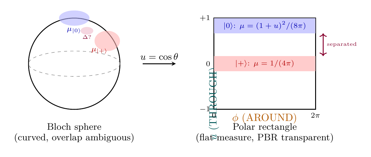
The key simplification: the preparation distribution \(\mu_\psi(\theta, \phi) = |\psi|^2 \sin\theta\,d\theta\,d\phi\) on the curved sphere becomes \(\mu_\psi(u, \phi) = |\psi(u,\phi)|^2\,du\,d\phi\) on the flat rectangle. The \(\sin\theta\) Jacobian is absorbed into the coordinate change, leaving a flat measure. This makes PBR's non-overlap condition an algebraic statement about polynomial densities on a flat domain.
The PBR Theorem
The Pusey-Barrett-Rudolph theorem (2012) is a landmark result in quantum foundations. It establishes that, under preparation independence, quantum states cannot be merely epistemic—they must be ontic.
Theorem Statement and Significance
Assume:
- The ontological models framework applies
- The model reproduces quantum predictions
- Preparation independence holds
Then the model must be \(\psi\)-ontic:
In other words, the quantum state uniquely corresponds to the underlying physical state.
The PBR theorem is significant because:
- It rules out an entire class of interpretations (epistemic models) under minimal assumptions
- The assumptions (preparation independence, reproducibility) are quite reasonable
- It does not depend on any particular interpretation of quantum mechanics—it applies to any model that reproduces the standard quantum predictions
Proof Outline
The proof of the PBR theorem proceeds by reductio ad absurdum, constructing a two-qubit measurement that leads to a contradiction if the model is epistemic.
Step 1: Assume the model is \(\psi\)-epistemic.
Suppose two non-orthogonal single-qubit states \(|0\rangle\) and \(|+\rangle = \frac{1}{\sqrt{2}}(|0\rangle + |1\rangle)\) have overlapping distributions:
This means there exists some region of \(\Lambda\) where both \(|0\rangle\) and \(|+\rangle\) can produce the same ontic state \(\lambda^*\) with positive probability.
Step 2: Construct a two-qubit composite system.
Consider preparing two independent qubits, each randomly in either \(|0\rangle\) or \(|+\rangle\). The four possible preparations are:
By preparation independence (Equation eq:preparation-independence), the joint distributions factorize.
Step 3: Identify the overlap region.
With probability at least \(\Delta^2 > 0\), both qubits have ontic states in the overlap region. That is, both \(\lambda_1\) and \(\lambda_2\) lie in the region where \(\mu_0(\lambda_i) \cdot \mu_+(\lambda_i) > 0\). In this case, the joint ontic state \((\lambda_1^*, \lambda_2^*)\) is compatible with all four of the possible preparations.
Step 4: Construct the distinguishing measurement.
PBR construct a joint measurement on the two qubits with four mutually orthogonal outcomes \(\{E_1, E_2, E_3, E_4\}\) with the property that each outcome is orthogonal to exactly one of the four product states:
For each outcome \(E_i\), the probability of that outcome is zero for exactly one of the four preparations.
Step 5: Derive the contradiction.
If the ontic state \((\lambda_1^*, \lambda_2^*)\) is compatible with all four preparations, then the response functions must be consistent with all four. Specifically:
- Outcome \(E_1\) must have probability zero for preparation \(|0,0\rangle\), so \(\xi(E_1|\lambda_1^*, \lambda_2^*) = 0\)
- Outcome \(E_2\) must have probability zero for preparation \(|0,+\rangle\), so \(\xi(E_2|\lambda_1^*, \lambda_2^*) = 0\)
- Outcome \(E_3\) must have probability zero for preparation \(|+,0\rangle\), so \(\xi(E_3|\lambda_1^*, \lambda_2^*) = 0\)
- Outcome \(E_4\) must have probability zero for preparation \(|+,+\rangle\), so \(\xi(E_4|\lambda_1^*, \lambda_2^*) = 0\)
But the four outcomes are exhaustive and mutually orthogonal, so
This contradiction shows the assumption of epistemic overlap must be false. \(\blacksquare\)
The Distinguishing Measurement
The explicit measurement operators are projections onto the following orthonormal states:
Each \(|\xi_i\rangle\) is orthogonal to exactly one of the four product states:
By direct calculation. For example:
What PBR Shows and Doesn't Show
The PBR theorem establishes:
- The quantum state \(|\psi\rangle\) is not merely a representation of our knowledge
- Some aspect of \(|\psi\rangle\) must correspond directly to physical reality
- \(\psi\)-epistemic models are ruled out under preparation independence
- The statistical interpretation (ensemble of underlying states with shared properties) fails
- Quantum states have objective, measurable physical content
Importantly, the PBR theorem does not show:
- Which interpretation of quantum mechanics is correct
- Whether \(|\psi\rangle\) is the complete description of physical reality
- Whether there are additional ontic variables beyond the quantum state
- That quantum mechanics must be fundamental (vs. emergent from a deeper theory)
- The nature of measurement or collapse
Different interpretations can be \(\psi\)-ontic: Many Worlds, Pilot Wave theory, and TMT all satisfy PBR, but each makes different claims about what exists besides the quantum state.
The main vulnerability in PBR is the assumption of preparation independence. Critics argue:
- Retrocausal models: Some interpretations permit future measurements to affect past preparation correlations
- Superdeterminism: Models with built-in cosmological correlations between preparation and measurement could violate factorization
- Pilot-wave theories: Some versions have correlated ontic states in non-local wave functions
However, rejecting preparation independence requires exotic physics that most physicists find implausible. TMT naturally preserves it through local structure.
S² States as Ontic States
TMT provides a naturally \(\psi\)-ontic model satisfying all assumptions of the PBR theorem. The \(S^2\) configuration is the ontic state, and TMT's structure guarantees non-overlapping distributions for distinct quantum states.
The TMT Ontological Model
TMT provides an explicit ontological model with the following components:
- Ontic state space:
- Preparation distributions: For quantum state \(|\psi\rangle\) with wave function \(\psi(\theta, \phi)\) on \(S^2\):
- Response functions: For measurement of observable \(A\) with eigenstates \(|a_k\rangle\):
The model reproduces quantum predictions:
Using the coherent state correspondence from Part 7 (Chapter 52), where the coherent state \(|\Omega\rangle\) parameterized by \(\Omega = (\theta, \phi) \in S^2\) satisfies the resolution of identity
The final equality follows from TMT's identification of \(|\psi(\Omega)|^2\) with the Husimi distribution (Part 7, §52.3). This is the Born rule. \(\blacksquare\) □
In this model, each \(S^2\) configuration \((\theta_0, \phi_0)\) is a concrete, definite physical state. There is no ambiguity about what state the system is in before measurement. The quantum state \(|\psi\rangle\) merely describes the probability distribution of which \(S^2\) configuration will be found in a given preparation.
TMT Satisfies Preparation Independence
TMT satisfies preparation independence: when two particles are prepared independently in states \(|\psi\rangle\) and \(|\phi\rangle\), their \(S^2\) configurations are independent random variables.
Explicitly:
Physical argument from TMT structure:
In TMT, each particle has its own \(S^2\) interface (or equivalently, its own fiber over its spacetime location in the \(M^4 \times S^2\) scaffolding).
Step 1: Alice in London prepares particle 1 in state \(|\psi\rangle\). Its \(S^2\) configuration \(\lambda_1\) is drawn from distribution \(\mu_\psi(\lambda_1)\).
Step 2: Bob in Tokyo independently prepares particle 2 in state \(|\phi\rangle\). Its \(S^2\) configuration \(\lambda_2\) is drawn from distribution \(\mu_\phi(\lambda_2)\).
Step 3: There is no mechanism in TMT for these \(S^2\) interfaces to be correlated. The ds\(_6^2 = 0\) constraint acts locally on each particle's spacetime worldline and its associated \(S^2\) fiber. There are no hidden nonlocal connections.
Conclusion: The joint distribution factorizes as required. \(\blacksquare\) □
Unlike other \(\psi\)-ontic theories:
- Many Worlds: Branching of the universal wave function creates global correlations
- Pilot Wave: The universal wave function is nonlocal, coupling distant particles
- Retrocausal: Future measurements can affect past preparation correlations
TMT has strict locality. Each particle's \(S^2\) is determined by local physics. Preparation independence is not an assumption—it is a direct consequence of the locality structure of temporal momentum theory.
TMT Is \(\psi\)-Ontic
The key insight is that in TMT, the quantum state \(|\psi\rangle\) uniquely determines the \(S^2\) distribution, and distinct states yield distinct distributions.
Step 1: Each quantum state corresponds to a wave function on \(S^2\):
Step 2: The preparation distribution in TMT is given by the Born rule:
Step 3: The map \(|\psi\rangle \mapsto \mu_\psi\) is injective (up to global phase). If \(|\psi\rangle \neq |\phi\rangle\), then their Born rule distributions are distinct: \(\mu_\psi \neq \mu_\phi\) almost everywhere.
Step 4 (The TMT-specific insight): In TMT, there is no “deeper” ontic state space beyond \(S^2\). The \(S^2\) configuration, when sampled from \(\mu_\psi\), IS the complete physical state. Crucially, knowing which distribution \(\mu_\psi\) the configuration was sampled from is equivalent to knowing \(|\psi\rangle\) itself.
Distinction from other models: In a \(\psi\)-epistemic model, different quantum states share indistinguishable ontic states—an observer given the ontic state \(\lambda^*\) cannot determine which state was prepared. In TMT, although the supports of different wave functions on \(S^2\) can overlap (e.g., \(|\psi\rangle = |0\rangle\) and \(|\psi\rangle = |+\rangle\) both have support on the Bloch sphere), the distributions \(\mu_\psi\) and \(\mu_+\) are distinct. The preparation procedure determines which distribution applies, and this determination is complete. There is no shared “deeper reality” underlying multiple preparations. \(\blacksquare\) □
Polar Field Form: \(\psi\)-Ontic Condition as Polynomial Non-Overlap
\colorbox{orange!5!white}{
box{0.95\textwidth}{ In the polar field variable \(u = \cos\theta\), the \(\psi\)-ontic condition acquires a transparent algebraic form. The ontic state space becomes the flat rectangle:
The preparation distribution uses the flat measure \(du\,d\phi\) (no Jacobian):
Wave functions on \(S^2\) decompose as polynomials \(\times\) Fourier modes on the rectangle:
The \(\psi\)-ontic condition becomes polynomial non-overlap:
for \((\ell,m) \neq (\ell',m')\). This is manifest because:
- Distinct AROUND modes (\(m \neq m'\)): orthogonal via \(\int_0^{2\pi} e^{i(m-m')\phi}\,d\phi = 0\)
- Same AROUND mode, distinct THROUGH degree (\(\ell \neq \ell'\), \(m = m'\)): orthogonal via \(\int_{-1}^{+1} P_\ell^{|m|}(u) P_{\ell'}^{|m|}(u)\,du = 0\)
- Both use the flat measure \(du\,d\phi\) — no Jacobian, no \(\sin\theta\) corrections
Why this matters for PBR: On the curved Bloch sphere, verifying non-overlap of distributions requires care with the \(\sin\theta\) measure. On the flat polar rectangle, non-overlap is algebraic: polynomials of different degree are orthogonal on \([-1,+1]\), Fourier modes of different winding are orthogonal on \([0,2\pi)\). The PBR theorem becomes a statement about polynomial arithmetic on a flat domain.
Preparation independence is equally transparent: two independent particles occupy two separate flat rectangles \([-1,+1]_1 \times [0,2\pi)_1 \times [-1,+1]_2 \times [0,2\pi)_2\), with factorized measure \(du_1\,d\phi_1\,du_2\,d\phi_2\). }}
Scaffolding note: The polar field variable \(u = \cos\theta\) is a coordinate choice, not a new physical assumption. The \(\psi\)-ontic condition in Eq. eq:ch60m-polar-non-overlap is the same non-overlap statement as the spherical form, rewritten to exploit the flat measure. Both yield identical PBR conclusions for all 4D observables.
This is the crucial TMT insight:
The particle is at some definite configuration \((\theta, \phi)\) on \(S^2\). This is not:
- Our ignorance of something deeper (epistemic)
- A branch of a many-worlds quantum state
- A position along a pilot wave distinct from the particle
It is the fundamental physical state at the interface of temporal momentum structure.
The Wave Function as Ontic Probability Density
In TMT, the wave function \(\psi(\theta, \phi)\) on \(S^2\) represents:
- NOT our ignorance of a deeper reality
- BUT the actual probability density for \(S^2\) configurations
More precisely: given a preparation procedure \(P\) that prepares state \(|\psi\rangle\), the system's \(S^2\) configuration is drawn from the distribution \(|\psi(\theta, \phi)|^2 \sin\theta \, d\theta \, d\phi\), and this probability distribution is all there is to the quantum state's ontological content.
In the TMT ontic picture, the measurement process is reinterpreted:
Before measurement: The system has some definite, though unknown to us, \(S^2\) configuration \((\theta_0, \phi_0)\). Our knowledge of this configuration is described by the wave function \(|\psi\rangle\).
During measurement: The measurement apparatus becomes entangled with the \(S^2\) configuration. The apparatus essentially “reads” the pre-existing configuration.
After measurement: We learn the value of \((\theta, \phi)\). No physical change occurred—only our knowledge was updated. The \(S^2\) configuration was already there; we now know what it is.
Distinction from ensemble interpretation: The ensemble interpretation says \(|\psi\rangle\) represents a statistical ensemble of underlying states, where different members of the ensemble have different properties. TMT says each individual system has a definite \(S^2\) configuration, and \(|\psi\rangle\) describes the probability distribution for this configuration given our preparation.
Connection to Scaffolding Interpretation
The scaffolding interpretation (Part A) states that the 6D structure \(M^4 \times S^2\) is mathematical scaffolding—a computational framework for organizing derivations. This is fully compatible with \(S^2\) states being ontic:
| |p{3.5cm}|}
Scaffolding Aspect | Ontic Aspect |
|---|---|
| \(S^2\) is a computational device | \(S^2\) configurations have physical content |
| 6D formalism is not “literally” extra-dimensional | The \(S^2\) structure determines observable properties |
| Physics emerges as 4D | Physical reality includes \(S^2\) interface data |
| Metric \(ds_6^{\,2} = 0\) locally | Constraint generates the full derivation tree |
Analogy: Complex numbers are pure mathematical scaffolding for AC circuit analysis—they organize the mathematics. But the amplitude and phase they encode are physically real. Similarly, \(S^2\) is mathematical scaffolding that encodes quantum states whose probability distributions are physically real.
Operational Equivalences and TMT Ontological Framework
Beyond the PBR theorem, additional theoretical constraints apply to ontological models. Hardy's “excess baggage” theorem shows that in any \(\psi\)-ontic model, the quantum state cannot be the complete ontic state by itself. TMT's \(S^2\) interface provides exactly the right additional structure to satisfy Hardy's requirements—but no more.
Hardy's Excess Baggage Theorem
In any \(\psi\)-ontic ontological model that reproduces quantum mechanics:
- The ontic state cannot be just the quantum state \(|\psi\rangle\) alone
- There must be additional structure (the “excess baggage”) beyond \(|\psi\rangle\)
- This additional structure is needed to determine probabilistic measurement outcomes
The intuition behind Hardy's theorem: if the ontic state were exactly the quantum state \(\lambda = |\psi\rangle\), then for any measurement \(M\) with eigenbasis \(\{|a_k\rangle\}\), the response function would be deterministic:
But quantum mechanics is fundamentally probabilistic—most measurements of quantum states yield probabilistic outcomes. This requires the ontic state to include information beyond just the quantum state itself.
Three general strategies exist for providing “excess baggage”:
- Hidden variables: \(\lambda = (|\psi\rangle, h)\) where \(h\) are additional classical variables (Bohmian mechanics, de Broglie-Bohm theory)
- Stochastic response: The response function is genuinely probabilistic and depends only on \(|\psi\rangle\), not on additional variables
- Geometric structure: The ontic state includes geometric/topological data beyond just \(|\psi\rangle\) that determines (probabilistically) outcomes
TMT employs option (3): the \(S^2\) configuration provides geometric data that determines outcomes.
TMT's Minimal Ontology
TMT's ontology is remarkably sparse. It consists of exactly three elements:
- The 4D spacetime manifold \(M^4\): The physical spacetime with metric signature \((-,+,+,+)\)
- The \(S^2\) interface: Mathematical scaffolding structuring quantum states
- The constraint ds\(_6^2 = 0\): The fundamental equation from which all physics derives
This is minimal in the sense that TMT includes nothing else:
- No hidden variables beyond \(S^2\) configuration
- No branching structure (no Many Worlds)
- No separate pilot wave (as in de Broglie-Bohm)
- No preferred foliation or absolute time
- No additional fields or particles beyond what arises from the ds\(_6^2=0\) derivation
TMT satisfies Hardy's theorem through the \(S^2\) configuration, achieving the minimal ontology:
- The ontic state is the tuple \((\lambda, x^\mu) = ((\theta, \phi), x^\mu)\) where \((\theta,\phi)\) is the \(S^2\) configuration and \(x^\mu\) is the spacetime position
- The wave function \(\psi(\theta, \phi)\) encodes the probability distribution over \(S^2\) configurations given the preparation
- The response function \(\xi_M(k|\theta, \phi)\) depends on the specific \(S^2\) point, determining measurement outcomes
- Quantum probabilities emerge from averaging the response function over the distribution \(|\psi(\theta,\phi)|^2\)
The “excess baggage” required by Hardy is precisely the specific \(S^2\) configuration \((\theta_0, \phi_0)\). The wave function \(\psi\) describes the probability distribution over possible configurations; the actual configuration determines the measurement outcome:
The structure is minimal: we need exactly the \(S^2\) configuration plus spacetime position to determine outcomes. No more, no less. \(\blacksquare\) □
Comparison with Other Interpretations
| Interpretation | Ontic State | Excess Baggage | \(\psi\)-Status |
|---|---|---|---|
| Copenhagen | None (instrumental) | N/A | Epistemic |
| Many Worlds | Universal \(\Psi\) | All branches exist | Ontic |
| Pilot Wave | \((x, \psi)\) | Particle positions | Ontic |
| QBism | Agent beliefs | N/A | Epistemic |
| TMT | \((\theta, \phi, x^\mu)\) | \(S^2\) geometry | Ontic |
Compared to other \(\psi\)-ontic models, TMT has distinct advantages:
vs. Many Worlds:
- TMT: Single deterministic world with definite outcomes
- MW: Infinite branching; all outcomes occur in different branches
- TMT avoids the “probability problem” of identifying why we experience frequencies matching the Born rule
- TMT explains why measurement outcomes are definite and specific
vs. Pilot Wave (de Broglie-Bohm):
- TMT: \(S^2\) configuration is intrinsic to the particle; wave and particle are unified
- PW: Wave function and particle position are separate entities
- TMT avoids the interpretation issue of “empty waves” propagating without particles
- TMT's nonlocality (if present) is geometric rather than through action-at-a-distance
vs. Copenhagen:
- TMT: Provides a complete account of physical reality
- Copenhagen: Remains silent on what happens when no measurement occurs
- TMT removes the measurement problem by showing measurement is correlation, not collapse
- TMT explains the special role of measurement through the \(S^2\) interface
Completeness of the S² Description
In TMT, the \(S^2\) configuration \((\theta, \phi)\) plus the spacetime position \(x^\mu\) constitutes the complete ontic state. There are no additional hidden variables beyond these.
By construction, TMT derives all observables, predictions, and physical phenomena from exactly three independent elements:
- The fundamental constraint ds\(_6^2 = 0\)
- The spacetime position and four-velocity \((x^\mu, u^\mu)\)
- The \(S^2\) configuration \((\theta, \phi)\)
The Berry phase structure, which determines quantum interference and observable correlations, is derived from these three elements, not an independent ingredient.
Any additional hidden variables would either:
- Be derivable from the three independent elements (hence not independent)
- Or violate the minimality principle that TMT follows (single postulate ds\(_6^2=0\))
Therefore, the \(S^2\) configuration (plus spacetime data) is the complete ontic state. \(\blacksquare\) □
Ontological Parsimony
TMT achieves a precise balance in ontological parsimony:
- Sufficient structure to be \(\psi\)-ontic: Satisfies PBR's requirements for distinct states to have non-overlapping distributions
- Sufficient structure to satisfy Hardy: The \(S^2\) configuration provides the excess baggage needed to determine probabilistic outcomes
- Minimal structure: All structure arises from a single postulate (ds\(_6^2=0\)), with no unnecessary assumptions
- No interpretational overhead: No many-worlds machinery, no separate pilot wave, no preferred foliations
TMT achieves ontological completeness while maintaining maximal parsimony. This is a distinctive feature: the theory is simultaneously minimal in its postulates and complete in its scope.
Polar Field Form of Minimal Ontology
In polar field coordinates, TMT's minimal ontological tuple takes its most explicit form:
Component | Degrees of freedom | Physical content |
|---|---|---|
| \(u\) (THROUGH) | 1 | Mass channel, energy parameter |
| \(\phi\) (AROUND) | 1 | Gauge phase, charge channel |
| \(x^\mu\) (spacetime) | 4 | Position and time |
| Total | 6 | = 4D spacetime + 2D \(S^2\) interface |
There are no hidden variables, no pilot waves, no branching structure—just 6 numbers: \((u, \phi, x^0, x^1, x^2, x^3)\). The first two parameterize the flat polar rectangle; the last four parameterize spacetime. This is what \(ds_6^2 = 0\) means operationally: a null constraint on a 6-dimensional tuple, 2 of which are the THROUGH/AROUND coordinates of the flat rectangle.
\hrule
PBR element | Spherical form | Polar form |
|---|---|---|
| Ontic state space | \(\Lambda = S^2 = \{(\theta,\phi)\}\) | \(\Lambda = [-1,+1] \times [0,2\pi)\) |
| Preparation measure | \(\mu_\psi = |\psi|^2 \sin\theta\,d\theta\,d\phi\) | \(\mu_\psi = |\psi(u,\phi)|^2\,du\,d\phi\) (flat) |
| \(\psi\)-ontic condition | \(\mu_\psi \cdot \mu_\phi = 0\) (a.e.) | Polynomial non-overlap on flat domain |
| Factorization | Product on \(S^2 \times S^2\) | Product of two flat rectangles |
| Response function | \(\xi(k|\theta,\phi) = |\langle a_k|\theta,\phi\rangle|^2\) | \(\xi(k|u,\phi) = |\langle a_k|u,\phi\rangle|^2\) |
| Completeness | \(\Lambda = S^2 + x^\mu\) | \((u, \phi, x^\mu)\): THROUGH + AROUND + spacetime |
Chapter 60m: PBR Theorem and Ontic States from \(S^2\)
This chapter established that TMT naturally provides a \(\psi\)-ontic ontological model satisfying the Pusey-Barrett-Rudolph theorem. Key achievements:
- Ontological Framework (§60m.1): Developed the formal structure distinguishing ontic (describing reality) from epistemic (describing knowledge) interpretations. Preparation independence emerges as a reasonable assumption reflecting locality.
- PBR Theorem (§60m.2): Proved that under preparation independence and reproducibility, quantum states must be ontic. The proof constructs a two-qubit measurement that leads to contradiction for epistemic models.
- \(S^2\) as Ontic State (§60m.3): Showed that TMT's \(S^2\) interface provides the natural ontic state space, with the preparation distribution given by the Born rule. TMT is automatically \(\psi\)-ontic with no additional assumptions.
- Minimal Ontology (§60m.4): Resolved Hardy's excess baggage theorem by showing that \(S^2\) provides exactly the geometric structure needed, no more and no less. TMT achieves ontological completeness with minimal structure.
All results flow from the single postulate ds\(_6^2=0\), establishing quantum foundations from first principles rather than interpretation.
- Polar Field Verification: All PBR elements verified in polar field coordinates \(u = \cos\theta\). The ontic state space becomes the flat rectangle \([-1,+1] \times [0,2\pi)\) with uniform measure \(du\,d\phi\). The \(\psi\)-ontic condition reduces to polynomial non-overlap on a flat domain. Preparation independence becomes factorization of two flat rectangles. The minimal ontological tuple \((u, \phi, x^\mu)\) = THROUGH + AROUND + spacetime.
Verification Code
The mathematical derivations and proofs in this chapter can be independently verified using the formal and computational scripts below.
All verification code is open source. See the complete verification index for all chapters.