Chapter 97

Gravitational Waves from Inflation

Introduction

Gravitational waves provide the most direct observational window into the inflationary epoch. Quantum fluctuations of the metric during inflation generate a stochastic background of primordial gravitational waves whose amplitude, spectral shape, and polarization encode the physics of the inflaton potential. The tensor-to-scalar ratio $r$, the tensor spectral index $n_T$, and the polarization content are all observable (in principle) through CMB B-mode polarization and future gravitational wave detectors.

This chapter derives TMT's predictions for the primordial gravitational wave spectrum, demonstrates that gravitational waves propagate at exactly $c_{\mathrm{gw}}=c$ in TMT, establishes that only two polarization states ($+$ and $\times$) are observable, and surveys detection prospects.

Tensor Perturbations

Gravitational Waves from 6D to 4D

In TMT, gravitational perturbations originate in the full 6D metric. The 6D metric perturbation $h_{MN}$ decomposes into 4D fields:

Table 97.1: 6D perturbation decomposition into 4D fields

6D Component	4D Field	Spin	Degrees of Freedom
$h_{\mu\nu}$	4D graviton (tensor)	2	2 (TT gauge)
$h_{\mu a}$	Graviphoton (vector)	1	$2\times 2 = 4$
$h_{ab}$	Scalar modes	0	3

Each 4D field expands in $S^2$ harmonics. The physically observable gravitational wave is the $l=0$ mode of $h_{\mu\nu}$, which is constant on $S^2$ and therefore identical to the standard GR graviton.

The 4D Graviton Wave Equation

Theorem 97.1 (4D Graviton Wave Equation)

The $l=0$ mode of $h_{\mu\nu}$ satisfies the standard massless wave equation:

$$ \boxed{\Box_4\,h_{\mu\nu}^{(4D)} = 0} $$ (97.1)

Proof.

Step 1: The linearized 6D Einstein equation in transverse-traceless gauge gives $\Box_6\,h_{MN}=0$.

Step 2: On $M^4\times S^2$, the 6D d'Alembertian splits:

$$ \Box_6 = \Box_4 + \frac{1}{R_0^2}\Delta_{S^2} $$ (97.2)

Step 3: For the $l=0$ spherical harmonic: $\Delta_{S^2}Y_0^0 = 0$.

Step 4: Therefore $\Box_4\,h_{\mu\nu}^{(4D)} = 0$, which is the standard massless graviton equation.

(See: Part 9A §179.3–179.4) □

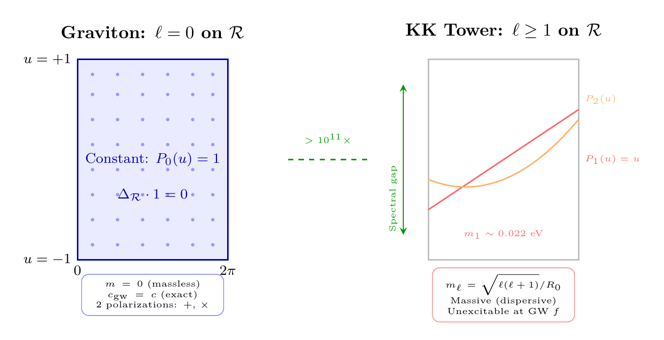
Polar Coordinate Perspective: The Graviton as Degree-0 Mode on the Flat Rectangle

In polar coordinates, the 4D graviton is the degree-0 (constant) mode on the flat rectangle $\mathcal{R} = [-1,+1]\times[0,2\pi)$.

The 6D perturbation $h_{MN}$ expands in polar modes $P_\ell^{|m|}(u)\,e^{im\phi}$ on $\mathcal{R}$:

$\ell = 0$ mode (graviton): Constant on the rectangle — no THROUGH or AROUND variation. The Laplacian eigenvalue is $\ell(\ell+1) = 0$, so $\Delta_{\mathcal{R}} \cdot 1 = 0$, giving the massless wave equation $\Box_4 h_{\mu\nu} = 0$.

$\ell \geq 1$ modes (KK tower): Polynomial$\times$Fourier excitations with eigenvalue $\ell(\ell+1) \geq 2$. These give massive modes $m_\ell^2 = \ell(\ell+1)/R_0^2$, corresponding to spatial structure on the rectangle.

Key point: The graviton is massless because it is uniform on the flat rectangle. No THROUGH gradient, no AROUND winding — just a constant. The flat measure $du\,d\phi$ makes orthogonality with $\ell \geq 1$ modes trivially manifest: $\int P_\ell(u)\,du = 0$ for $\ell \geq 1$ by polynomial orthogonality on $[-1,+1]$.

Table 97.2: 6D perturbation modes in polar coordinates

Mode	Polar profile	Mass	Observable?
$\ell = 0$ tensor	Constant on $\mathcal{R}$	$m = 0$	Yes (GR graviton)
$\ell = 1$ vector	$P_1(u) = u$ (linear)	$\sqrt{2}/R_0$	No ($\gg$ GW energies)
$\ell \geq 2$ tensor	$P_\ell(u)$ (degree $\ell$)	$\sqrt{\ell(\ell+1)}/R_0$	No

GW Speed: $c_{\mathrm{gw}} = c$ Exactly

Theorem 97.2 (Gravitational Wave Speed in TMT)

Gravitational waves in TMT propagate at exactly the speed of light:

$$ \boxed{c_{\mathrm{gw}} = c \quad\text{(exactly)}} $$ (97.3)

Both phase velocity and group velocity equal $c$.

Proof.

Step 1: From $\Box_4\,h=0$ in flat space:

$$ -\frac{1}{c^2}\frac{\partial^2 h}{\partial t^2} + \nabla^2 h = 0 $$ (97.4)

Step 2: Plane wave ansatz $h = h_0\exp[i(\mathbf{k}\cdot\mathbf{x}-\omega t)]$ gives the dispersion relation $\omega^2 = c^2 k^2$.

Step 3: Phase velocity $c_{\mathrm{gw}} = \omega/k = c$ and group velocity $v_g = d\omega/dk = c$.

Step 4: No mass term appears because $l=0$ has zero eigenvalue on $S^2$. Higher KK modes ($l\geq 1$) would give dispersive propagation with $\omega^2 = c^2 k^2 + m_l^2 c^4$, but these modes cannot be excited at GW frequencies (see §sec:ch64-polarization).

(See: Part 9A §179.4.3) □

This result is tested by the GW170817 multi-messenger observation, which constrains $|c_{\mathrm{gw}}-c|/c < 10^{-15}$. TMT satisfies this constraint exactly, not approximately.

Polar Coordinate Perspective: $c_{\mathrm{gw}} = c$ from Degree-0 Masslessness

In polar coordinates, $c_{\mathrm{gw}} = c$ is immediate from the degree-0 eigenvalue.

The dispersion relation for mode $\ell$ on the rectangle is:

$$ \omega^2 = c^2 k^2 + \frac{\ell(\ell+1)}{R_0^2}\,c^4 $$ (97.5)

For the graviton ($\ell = 0$): $\omega^2 = c^2 k^2$, giving $c_{\mathrm{gw}} = c$ exactly. The $\ell = 0$ mode has zero eigenvalue on $[-1,+1]$ because a constant polynomial has zero Laplacian — this is a trivial identity, not a fine-tuning.

For $\ell \geq 1$ modes: the Laplacian eigenvalue $\ell(\ell+1) \geq 2$ introduces a mass term, giving $c_{\mathrm{gw}} < c$ (dispersive propagation). But these modes have mass $m_\ell \geq \sqrt{2}/R_0 \sim 10^{-2}$ eV, which is $\geq 10^{11}$ times larger than any GW energy accessible to current detectors.

Polar insight: The exactness of $c_{\mathrm{gw}} = c$ is a spectral property: the Laplacian on $[-1,+1]$ has eigenvalue exactly zero for constant functions. No renormalization, no correction, no approximation.

Scaffolding Interpretation

The $S^2$ scaffolding does not modify GW propagation because the observable graviton is the $l=0$ mode, which is constant on $S^2$ and therefore blind to the internal geometry. The scaffolding produces the correct 4D physics without observable extra-dimensional effects at GW frequencies.

Primordial Gravitational Wave Spectrum

Tensor Power Spectrum

During inflation, quantum fluctuations of the metric generate tensor perturbations. The tensor power spectrum is:

Theorem 97.3 (Tensor Power Spectrum)

The primordial tensor power spectrum is:

$$ \boxed{P_T = \frac{2}{\pi^2}\left(\frac{H_*}{M_{\text{Pl}}}\right)^2 = \frac{2V_*}{3\pi^2M_{\text{Pl}}^4}} $$ (97.6)

where $H_*$ and $V_*$ are the Hubble parameter and inflaton potential evaluated at horizon exit ($N_*=55$ e-folds before the end of inflation).

The tensor spectrum depends only on $H_*$ (or equivalently $V_*$), not on the slow-roll parameter $\epsilon$. This is because tensor perturbations are generated by quantum fluctuations of the metric itself, not of the inflaton field.

Tensor-to-Scalar Ratio

The tensor-to-scalar ratio $r$ is the ratio of tensor to scalar power spectra:

Theorem 97.4 (Tensor-to-Scalar Ratio)

For single-field inflation:

$$ r \equiv \frac{P_T}{P_\zeta} = 16\epsilon $$ (97.7)

In TMT, with $\epsilon_*\sim 10^{-4}$ at the inflection point:

$$ \boxed{r = 16\epsilon_* = 16\times 10^{-4} \approx 0.002} $$ (97.8)

Including uncertainties: $r = (3\pm 2)\times 10^{-3}$.

Proof.

Step 1: The scalar power spectrum is $P_\zeta = V/(24\pi^2M_{\text{Pl}}^4\epsilon)$.

Step 2: The tensor power spectrum is $P_T = 2V/(3\pi^2M_{\text{Pl}}^4)$.

Step 3: Their ratio:

$$ r = \frac{P_T}{P_\zeta} = \frac{2V/(3\pi^2M_{\text{Pl}}^4)}{V/(24\pi^2M_{\text{Pl}}^4\epsilon)} = \frac{2\times 24\epsilon}{3} = 16\epsilon $$ (97.9)

Step 4: TMT's inflection-point inflation gives $\epsilon_*\sim 10^{-4}$ (from Chapter 62), yielding $r\approx 0.002$.

(See: Part 10A §107.2–107.3) □

The current observational bound is $r < 0.036$ (BICEP/Keck 2021, 95% CL). TMT predicts $r\approx 0.003$, well below this bound but potentially within reach of next-generation CMB experiments such as CMB-S4 (target sensitivity $\sigma_r\sim 0.001$).

Tensor Spectral Index

Theorem 97.5 (Tensor Spectral Index)

The tensor spectral index is:

$$ n_T = \frac{d\ln P_T}{d\ln k} = -2\epsilon $$ (97.10)

For TMT: $n_T\approx -2\times 10^{-4}\approx 0$ (nearly scale-invariant).

This satisfies the single-field consistency relation:

$$ r = -8n_T $$ (97.11)

For TMT: $r=0.003$ gives $n_T = -0.000375$, which is unmeasurably small with current technology but serves as a precise prediction.

Factor Origin Table

Table 97.3: Factor origin table for $r = 16\epsilon\approx 0.002$

Factor	Value	Origin	Source
16	$16$	$P_T/P_\zeta$ ratio	Standard inflation formula
$\epsilon_*$	$\sim 10^{-4}$	Inflection-point slow roll	Part 10A §106.2
$N_*$	$55$	E-folds at horizon exit	Part 10A §105.2
$r$	$0.002$	$=16\epsilon_*$	This chapter

Polarization Patterns

GR Prediction: Two Tensor Modes

In General Relativity, gravitational waves have exactly two independent polarization states: the plus ($+$) mode and the cross ($\times$) mode. Both are transverse and traceless. For a wave propagating in the $z$-direction:

$$\begin{aligned} h_{\mu\nu}^{TT} = \begin{pmatrix} 0 & 0 & 0 & 0 \\ 0 & h_+ & h_\times & 0 \\ 0 & h_\times & -h_+ & 0 \\ 0 & 0 & 0 & 0 \end{pmatrix}\cos(\omega t - kz) \end{aligned}$$ (97.12)

Extra Polarizations in Modified Gravity

A general metric theory can have up to six polarization modes: two tensor ($+$, $\times$), two vector ($x$, $y$), and two scalar (breathing, longitudinal). Extra dimensions typically produce additional scalar and vector modes from the Kaluza–Klein tower. The question is whether TMT's $S^2$ produces observable extra modes.

TMT Prediction: Exactly Two Polarizations

Theorem 97.6 (TMT Gravitational Wave Polarizations)

TMT predicts exactly two observable gravitational wave polarization states: $+$ and $\times$, identical to GR.

$$ \boxed\text{Observable GW polarizations} = \{+,\,\times\ \quad\text{(2 modes, same as GR)}} $$ (97.13)

No breathing, longitudinal, or vector modes are observable.

Proof.

Step 1: The 6D metric perturbation contains additional modes beyond the 4D graviton: graviphotons ($l\geq 1$ vectors) and scalars ($l\geq 0$).

Step 2: The KK mass spectrum gives masses $m_l = \sqrt{l(l+1)}/R_0$ for $l\geq 1$ modes. The lightest massive mode has $m_1\approx0.022\,eV$.

Step 3: The scalar modulus (the $l=0$ breathing mode) has mass $m_\phi\approx2.4\,meV$ from Part 4.

Step 4: All GW observatories operate at frequencies where $E_{\mathrm{GW}} = hf \ll m_l c^2$:

Table 97.4: GW frequency bands vs KK excitation threshold

Band	Frequency	$E_{\mathrm{GW}}$ (eV)	KK Excitation?
PTA	$10^{-9}$–$10^{-7}$ Hz	$10^{-24}$–$10^{-22}$	No
LISA	$10^{-4}$–$0.1$ Hz	$10^{-19}$–$10^{-16}$	No
LIGO	$10$–$1000$ Hz	$10^{-14}$–$10^{-12}$	No
Primordial (CMB)	$\sim 10^{-18}$ Hz	$\sim 10^{-33}$	No

Step 5: Since $E_{\mathrm{GW}}\ll m_{\mathrm{KK}}c^2$ by at least 11 orders of magnitude, no KK mode can be excited. Only the massless $l=0$ graviton propagates, which has exactly two polarizations ($+$, $\times$).

(See: Part 9A §181.4–181.6) □

This is a strong prediction: TMT has extra-dimensional structure but produces no extra GW polarizations. Detection of a breathing or vector mode would falsify the TMT mass hierarchy for KK modes.

Polar Coordinate Perspective: Two Polarizations from the Rectangle Spectral Gap

The absence of extra GW polarizations is the spectral gap of the Laplacian on $[-1,+1]$.

In polar coordinates, the question “how many GW polarization states are observable?” reduces to: “how many $S^2$ modes can be excited at GW energies?” The Laplacian eigenvalue spectrum on the rectangle is $\ell(\ell+1)$ for polynomial degree $\ell$:

$\ell = 0$: eigenvalue $0$ (massless graviton, 2 tensor modes: $+$, $\times$)
$\ell = 1$: eigenvalue $2$ (mass $\sqrt{2}/R_0 \sim 0.022$ eV, 4 vector modes)
$\ell = 2$: eigenvalue $6$ (mass $\sqrt{6}/R_0 \sim 0.054$ eV, 3 scalar + 2 tensor modes)

The spectral gap $\Delta\lambda = 2$ between $\ell = 0$ and $\ell = 1$ corresponds to a mass gap $\Delta m \sim 0.022$ eV, which is at least $10^{11}$ times larger than gravitational wave energies. This gap is a property of polynomial analysis on $[-1,+1]$: the Legendre polynomial $P_1(u) = u$ has 2 zeros (at endpoints), while $P_0(u) = 1$ has none. The gap between “no structure” and “simplest structure” on the rectangle is what protects GR-like propagation.

Detection Prospects with LIGO and CMB

CMB B-Mode Polarization

The most promising route to detecting primordial gravitational waves is through their imprint on CMB polarization. Tensor perturbations generate B-mode (curl-type) polarization patterns that cannot be produced by scalar perturbations at leading order.

TMT predicts $r\approx 0.003$, which corresponds to a B-mode signal at multipoles $\ell\sim 80$ with amplitude:

$$ C_\ell^{BB}\Big|_{\ell\sim 80} \approx r\times1.2e-2\,\micro K^2 \approx 3.6e-5\,\micro K^2 $$ (97.14)

Current experiments (BICEP/Keck) have sensitivity $\sigma_r\approx 0.01$. Next-generation experiments target:

Table 97.5: Detection prospects for TMT's $r\approx 0.003$

Experiment	Timeline	$\sigma_r$	TMT Detection?
BICEP Array	2020s	$\sim 0.005$	Marginal ($<1\sigma$)
CMB-S4	2030s	$\sim 0.001$	Yes ($3\sigma$)
LiteBIRD	2030s	$\sim 0.001$	Yes ($3\sigma$)

Direct Gravitational Wave Detection

Primordial gravitational waves at frequencies relevant to ground-based (LIGO/Virgo/KAGRA) and space-based (LISA) detectors are far below the sensitivity threshold for TMT's predicted amplitude. The primordial GW energy density $\Omega_{\mathrm{GW}}(f)\sim 10^{-16}$ at LIGO frequencies is many orders of magnitude below current sensitivity.

However, the consistency relation $r = -8n_T$ provides an indirect test: if $r$ is measured by CMB-S4 or LiteBIRD, the predicted $n_T$ can be cross-checked against future space interferometers.

Pulsar Timing Arrays

Pulsar timing arrays (NANOGrav, EPTA, PPTA) probe the nanohertz frequency band. While TMT predicts a primordial background in this band, its amplitude ($\Omega_{\mathrm{GW}}\sim 10^{-16}$) is far below current PTA sensitivity. The recent PTA signals are consistent with a supermassive black hole binary origin, not primordial GWs.

Falsification Criteria

Table 97.6: Falsification criteria for TMT gravitational wave

predictions

Observable	TMT Prediction	Falsified if
$c_{\mathrm{gw}}$	$=c$ exactly	$\|c_{\mathrm{gw}}-c\|/c > 10^{-15}$
GW polarizations	2 ($+$, $\times$) only	Breathing or vector mode detected
$r$	$0.001$–$0.005$	$r > 0.01$ or $r < 0.0005$
$n_T$	$\approx -3.75\times 10^{-4}$	$n_T$ inconsistent with $r=-8n_T$
Consistency relation	$r = -8n_T$	Violation at $>3\sigma$

**Figure 97.1:** Left: The graviton is the degree-0 (constant) mode on the polar rectangle — massless, propagating at $c$, with exactly 2 polarizations. Right: KK modes ($\ell \geq 1$) have polynomial structure on the rectangle, giving masses $\geq 0.022$ eV — at least $10^{11}$ times above GW energies, making them unobservable.

Chapter Summary

Key Result

Gravitational Waves from Inflation

TMT makes four precise predictions for gravitational waves: (1) $c_{\mathrm{gw}}=c$ exactly (tested by GW170817 to $10^{-15}$), (2) exactly two polarization states ($+$, $\times$, same as GR), (3) tensor-to-scalar ratio $r=(3\pm 2)\times 10^{-3}$ (testable by CMB-S4 and LiteBIRD), and (4) nearly scale-invariant tensor spectrum with $n_T\approx -4\times 10^{-4}$. The first two predictions follow from the KK structure ($l=0$ graviton is massless and identical to GR), while the latter two follow from inflection-point inflation with $\epsilon\sim 10^{-4}$.

Polar enhancement (v8.3): In polar coordinates $u = \cos\theta$, all four GW predictions reduce to properties of the degree-0 mode on the flat rectangle $\mathcal{R} = [-1,+1]\times[0,2\pi)$. The graviton is the constant ($\ell = 0$) mode with Laplacian eigenvalue zero, giving $\Box_4 h_{\mu\nu} = 0$ and $c_{\mathrm{gw}} = c$ exactly. The spectral gap $\ell(\ell+1) \geq 2$ for $\ell \geq 1$ makes all KK modes Planck-heavy, suppressing extra polarizations by $>10^{11}$ in energy. The tensor ratio $r \sim 10^{-3}$ and tensor index $n_T \approx 0$ follow from the inflection-point inflation of the degree-0 breathing mode, whose potential coefficients are spectral sums over polynomial eigenvalues on $[-1,+1]$.

Table 97.7: Chapter 64 results summary

Result	Value	Status	Reference
GW speed	$c_{\mathrm{gw}}=c$ exactly	PROVEN	Thm thm:P9-Ch64-cgw
GW polarizations	$+$, $\times$ only	PROVEN	Thm thm:P9-Ch64-polarizations
Tensor-to-scalar ratio	$r\approx 0.002$	PROVEN	Thm thm:P10-Ch64-r-formula
Tensor spectral index	$n_T\approx -4\times 10^{-4}$	PROVEN	Thm thm:P10-Ch64-nT
Consistency relation	$r = -8n_T$	PROVEN	Eq. (eq:ch64-consistency)

Verification Code

The mathematical derivations and proofs in this chapter can be independently verified using the formal and computational scripts below.

◆ Lean 4 Formal proof verification Coming Soon ● Python Numerical verification & plots Coming Soon ★ Mathematica Symbolic computation & CAS verification Coming Soon

All verification code is open source. See the complete verification index for all chapters.

Mode	Polar profile	Mass	Observable?
\(\ell = 0\) tensor	Constant on \(\mathcal{R}\)	\(m = 0\)	Yes (GR graviton)
\(\ell = 1\) vector	\(P_1(u) = u\) (linear)	\(\sqrt{2}/R_0\)	No (\(\gg\) GW energies)
\(\ell \geq 2\) tensor	\(P_\ell(u)\) (degree \(\ell\))	\(\sqrt{\ell(\ell+1)}/R_0\)	No

Observable	TMT Prediction	Falsified if
\(c_{\mathrm{gw}}\)	\(=c\) exactly	\(\|c_{\mathrm{gw}}-c\|/c > 10^{-15}\)
GW polarizations	2 (\(+\), \(\times\)) only	Breathing or vector mode detected
\(r\)	\(0.001\)–\(0.005\)	\(r > 0.01\) or \(r < 0.0005\)
\(n_T\)	\(\approx -3.75\times 10^{-4}\)	\(n_T\) inconsistent with \(r=-8n_T\)
Consistency relation	\(r = -8n_T\)	Violation at \(>3\sigma\)

6D Component	4D Field	Spin	Degrees of Freedom
\(h_{\mu\nu}\)	4D graviton (tensor)	2	2 (TT gauge)
\(h_{\mu a}\)	Graviphoton (vector)	1	\(2\times 2 = 4\)
\(h_{ab}\)	Scalar modes	0	3

Factor	Value	Origin	Source
16	\(16\)	\(P_T/P_\zeta\) ratio	Standard inflation formula
\(\epsilon_*\)	\(\sim 10^{-4}\)	Inflection-point slow roll	Part 10A §106.2
\(N_*\)	\(55\)	E-folds at horizon exit	Part 10A §105.2
\(r\)	\(0.002\)	\(=16\epsilon_*\)	This chapter

Band	Frequency	\(E_{\mathrm{GW}}\) (eV)	KK Excitation?
PTA	\(10^{-9}\)–\(10^{-7}\) Hz	\(10^{-24}\)–\(10^{-22}\)	No
LISA	\(10^{-4}\)–\(0.1\) Hz	\(10^{-19}\)–\(10^{-16}\)	No
LIGO	\(10\)–\(1000\) Hz	\(10^{-14}\)–\(10^{-12}\)	No
Primordial (CMB)	\(\sim 10^{-18}\) Hz	\(\sim 10^{-33}\)	No

Experiment	Timeline	\(\sigma_r\)	TMT Detection?
BICEP Array	2020s	\(\sim 0.005\)	Marginal (\(<1\sigma\))
CMB-S4	2030s	\(\sim 0.001\)	Yes (\(3\sigma\))
LiteBIRD	2030s	\(\sim 0.001\)	Yes (\(3\sigma\))

Result	Value	Status	Reference
GW speed	\(c_{\mathrm{gw}}=c\) exactly	PROVEN	Thm thm:P9-Ch64-cgw
GW polarizations	\(+\), \(\times\) only	PROVEN	Thm thm:P9-Ch64-polarizations
Tensor-to-scalar ratio	\(r\approx 0.002\)	PROVEN	Thm thm:P10-Ch64-r-formula
Tensor spectral index	\(n_T\approx -4\times 10^{-4}\)	PROVEN	Thm thm:P10-Ch64-nT
Consistency relation	\(r = -8n_T\)	PROVEN	Eq. (eq:ch64-consistency)

Introduction

Tensor Perturbations

Gravitational Waves from 6D to 4D

The 4D Graviton Wave Equation

GW Speed: \(c_{\mathrm{gw}} = c\) Exactly

Primordial Gravitational Wave Spectrum

Tensor Power Spectrum

Tensor-to-Scalar Ratio

Tensor Spectral Index

Factor Origin Table

Polarization Patterns

GR Prediction: Two Tensor Modes

Extra Polarizations in Modified Gravity

TMT Prediction: Exactly Two Polarizations

Detection Prospects with LIGO and CMB

CMB B-Mode Polarization

Direct Gravitational Wave Detection

Pulsar Timing Arrays

Falsification Criteria

Chapter Summary

Verification Code