The CKM Matrix
Introduction
The Cabibbo–Kobayashi–Maskawa (CKM) matrix describes quark flavor mixing in the weak interaction. In the Standard Model, its four independent parameters (three mixing angles and one CP-violating phase) are free parameters extracted from experiment. TMT derives the entire CKM matrix from the \(S^2\) scaffolding geometry, with zero free parameters.
The key mechanism is the misalignment between up-type and down-type quark localization on \(S^2\): because the c-parameters differ between the up and down sectors (\(c_u\neq c_d\), \(c_c\neq c_s\), \(c_t\neq c_b\)), the rotations needed to diagonalize the up-type and down-type mass matrices are different, and the CKM matrix measures this difference.
This chapter builds on the fermion mass results of Chapters 36–42. The localization parameters derived there determine the quark masses, and the same parameters, combined with \(S^2\) wavefunction overlaps, determine the CKM matrix elements.
Quark Flavor Mixing
The CKM Matrix: Definition and Physical Meaning
The CKM matrix relates the mass eigenstates of quarks to the weak interaction eigenstates:
The matrix \(V_{\mathrm{CKM}}\) is unitary (\(V^\dagger V = \mathbb{1}\)) and has four physical parameters: three mixing angles \(\theta_{12},\theta_{23},\theta_{13}\) and one CP-violating phase \(\delta\).
The TMT Origin: Misalignment of Up and Down Sectors
In TMT, the Yukawa matrices are determined by wavefunction overlaps on \(S^2\):
The left-handed wavefunctions are the \(\ell=1\) spherical harmonics:
The CKM matrix then arises as:
The c-Parameter Misalignment
The localization parameters for all six quarks (derived in Chapters 40–41) are:
| Generation | \(c_{\mathrm{up}}\) | \(c_{\mathrm{down}}\) | \(\Delta c = c_d - c_u\) | Physical effect |
|---|---|---|---|---|
| 1st (\(u\), \(d\)) | 1.3990 | 1.3372 | \(-0.0618\) | Small misalignment |
| 2nd (\(c\), \(s\)) | 0.8913 | 1.0991 | \(+0.2078\) | Moderate misalignment |
| 3rd (\(t\), \(b\)) | 0.5007 | 0.7967 | \(+0.2960\) | Largest misalignment |
The increasing \(|\Delta c|\) from 1st to 3rd generation reflects the fact that heavier quarks are more localized on \(S^2\) (smaller \(c\)), and the up–down mass splitting grows with generation.
The Fritzsch Texture from \(S^2\) Orthogonality
The explicit evaluation of the overlap integrals reveals that the Yukawa matrices have a specific texture structure. The key result is that the 1-2 direct coupling vanishes:
This vanishes exactly because \(Y_{1,0}\) (\(m=0\)) and \(Y_{1,+1}\) (\(m=+1\)) are orthogonal on \(S^2\). Similarly, the 1-3 coupling vanishes (\(m=0\) vs \(m=-1\)), and the 2-3 coupling vanishes (\(m=+1\) vs \(m=-1\)).
The vanishing of off-diagonal Yukawa elements is a mathematical consequence of spherical harmonic orthogonality on the \(S^2\) scaffolding. This derives the Fritzsch texture zeros from geometry rather than assuming them as a symmetry ansatz.
The resulting Yukawa matrix has the Fritzsch form:
Despite the diagonal Yukawa matrices, mixing still occurs because the up-type and down-type matrices have different eigenvalues (different c-parameters). The CKM matrix measures the misalignment between the rotations that diagonalize \(Y^{(u)}\) and \(Y^{(d)}\).
The CKM Elements
The Cabibbo Angle: \(V_{us}\)
The dominant CKM mixing angle is the Cabibbo angle \(\theta_C\), governing 1st–2nd generation mixing. TMT derives this from the down-type quark mass ratio via a 16-step derivation.
Step 1: Mass matrix structure. From the \(S^2\) overlap integrals (Eq. eq:ch43-Fritzsch-texture), the down-type mass matrix in the 1-2 sector has the Fritzsch form:
Step 2: Extract the 1-2 generation submatrix. For the 1-2 sector, the 3rd generation decouples to leading order:
Step 3: Compute \(MM^\dagger\) to extract mass eigenvalues.
Step 4: Perform the matrix multiplication.
Step 5: Find eigenvalues by solving the characteristic equation.
Step 6: Expand the determinant.
Step 7: Simplify to quadratic form.
Step 8: Apply the quadratic formula and expand for hierarchy. For \(|A_d| \ll |D_d|\):
Step 9: Extract mass values.
Step 10: Compute the mass ratio.
Step 11: Find the diagonalizing rotation angle. The mixing angle \(\theta^{(d)}_{12}\) that diagonalizes \(MM^\dagger\) satisfies:
Step 12: Apply small angle approximation. For small angles, \(\tan(2\theta) \approx 2\theta\):
Step 13: Express in terms of mass ratio. From Step 10, \(|A_d|/|D_d| = \sqrt{m_d/m_s}\):
Step 14: Include up-sector contribution. The up-type sector contributes analogously:
Step 15: Combine both sectors. The CKM Cabibbo angle receives contributions from both sectors:
Step 16: Numerical evaluation. Using the PDG 2024 running masses at \(\mu=2\,GeV\):
Comparison with experiment: \(\sin\theta_C^{\mathrm{obs}} = 0.22500\pm 0.00067\).
Agreement: \(|0.2242 - 0.2250|/0.0007 = 1.1\sigma\). \quad \(\blacksquare\)
(See: Part 6B §92, Part 6B §91.4–91.6) □
| Factor | Value | Origin | Source |
|---|---|---|---|
| \(m_d\) | \(4.70\,MeV\) | Down quark mass from \(c_d=1.337\) | Ch 41 |
| \(m_s\) | \(93.5\,MeV\) | Strange quark mass from \(c_s=1.099\) | Ch 41 |
| \(\sqrt{\phantom{x}}\) | — | Fritzsch texture eigenvalue relation | Part 6B §92 |
| \(\sin\theta_C\) | 0.2242 | \(=\sqrt{m_d/m_s}\) | This theorem |
The CP-Violating Phase: \(\delta\)
The CP-violating phase of the CKM matrix is:
Step 1: The Jarlskog invariant as basis-independent measure. CP violation is encoded in the basis-independent Jarlskog invariant:
Step 2: Relation to standard CKM parameters. In the standard parametrization with angles \(\theta_{12},\theta_{23},\theta_{13}\) and phase \(\delta\):
Step 3: The commutator formula for \(J\) from mass matrices. \(J\) can be computed directly without using CKM parameters:
Step 4: Generation phase assignment on \(S^2\). The three generations occupy different \(Y_{1,m}\) modes: Generation 1 (\(u,d\)) has \(m=0\) (real wavefunction), Generation 2 (\(c,s\)) has \(m=+1\) (phase \(e^{+i\phi}\)), and Generation 3 (\(t,b\)) has \(m=-1\) (phase \(e^{-i\phi}\)). The angular separation is \(2\pi/3 = 120^\circ\) between consecutive pairs.
Step 5: Fritzsch texture with phases from \(Y_{1,m}\) modes. From the \(S^2\) overlap integrals, the down-type mass matrix carries phases from the generation wavefunctions:
Step 6: Computing phase connections between generations. The Yukawa element connecting generations \(\alpha\) and \(\beta\) carries the phase:
Step 7: Dominant path in the commutator trace. The dominant contribution to \(\mathrm{Im}(\mathrm{Tr}[H_u, H_d]^3)\) comes from the path involving generations 1\(\to 2\to 3\):
Step 8: Geometric factor from spherical harmonic separation.
Step 9: Computing \(J\) from commutator with PDG 2024 masses. Substituting all six quark masses into Eq. (eq:ch43-J-commutator):
Step 10: Extracting \(\sin\delta\) from the Jarlskog invariant. From Eq. (eq:ch43-J-standard), solve for \(\sin\delta\):
Step 11: Computing the denominator using derived CKM parameters. From previous theorems: \(s_{12} = 0.2242\), \(s_{23} = 0.0410\), \(s_{13} = 0.00353\).
Step 12: Final calculation of \(\delta\).
Observed (PDG 2024): \(\delta = 65.4^\circ \pm 3.4^\circ\).
Agreement: \(|69.6^\circ - 65.4^\circ|/\sqrt{8^2+3.4^2} = 4.2^\circ/8.7^\circ = 0.5\sigma\). \quad \(\blacksquare\)
(See: Part 6B §93.1, Part 6B §91.3–91.6) □
The \(V_{cb}\) Element
The CKM element \(|V_{cb}|\) is:
Step 1: The 2-3 sector mixing. Following the same Fritzsch diagonalization procedure as for the Cabibbo angle, but now in the 2-3 generation sector:
Step 2: Up-sector contribution.
Step 3: Interference with CP phase. The CKM element receives contributions from both sectors with a relative phase \(\delta\):
Step 4: Numerical evaluation. Using \(\delta = 69.6^\circ\) (\(\cos 69.6^\circ = 0.347\)):
Observed (PDG 2024): \(|V_{cb}| = 0.04182\pm 0.00086\).
Agreement: \(0.2\sigma\). \quad \(\blacksquare\)
(See: Part 6B §93.2) □
The \(V_{ub}\) Element
Step 1: Wolfenstein parameters from derived quantities. From the preceding derivations:
Step 2: Numerical evaluation.
Observed (PDG 2024): \(|V_{ub}| = 0.00369\pm 0.00011\).
Agreement: \(1.5\sigma\). \quad \(\blacksquare\)
(See: Part 6B §93.3) □
The Complete Nine-Element CKM Matrix
The nine elements are determined by the four independent parameters \(\theta_{12},\theta_{23},\theta_{13},\delta\), all derived above. The remaining elements follow from the standard parametrization and unitarity:
| Element | TMT Formula | TMT Value | PDG 2024 | Agreement |
|---|---|---|---|---|
| \(|V_{ud}|\) | \(\sqrt{1-\lambda^2}\) | 0.9749 | 0.97435 | 99.9% |
| \(|V_{us}|\) | \(\sqrt{m_d/m_s}\) | 0.2242 | 0.22500 | 99.6% |
| \(|V_{ub}|\) | \(A\lambda^3\sqrt{\rho^2+\eta^2}\) | 0.00353 | 0.00369 | 95.7% |
| \(|V_{cd}|\) | \(\lambda\) | 0.2242 | 0.22486 | 99.8% |
| \(|V_{cs}|\) | \(\sqrt{1-\lambda^2}\) | 0.9749 | 0.97349 | 99.9% |
| \(|V_{cb}|\) | \(\sqrt{m_s/m_b}\times f_\phi\) | 0.0410 | 0.04182 | 98.1% |
| \(|V_{td}|\) | \(A\lambda^3(1-\rho)\) | 0.00822 | 0.00857 | 95.9% |
| \(|V_{ts}|\) | \(A\lambda^2\) | 0.0410 | 0.04110 | 99.8% |
| \(|V_{tb}|\) | \(\sqrt{1-A^2\lambda^4}\) | 0.99916 | 0.999118 | 99.99% |
All nine elements agree with experiment at the 96–100% level. The largest deviation is \(|V_{ub}|\) at \(1.5\sigma\), well within theoretical uncertainties. \quad \(\blacksquare\)
(See: Part 6B §94.1) □
Unitarity Triangle
Unitarity Verification
The CKM matrix must satisfy \(V^\dagger V = \mathbb{1}\). This provides a powerful consistency check on the TMT derivation.
First row unitarity:
First column unitarity:
Third row unitarity:
All rows and columns satisfy unitarity to better than \(0.1\%\), confirming the internal consistency of the derivation.
The Unitarity Triangle
The orthogonality condition between the first and third columns defines the “unitarity triangle”:
Dividing by \(V_{cd}V_{cb}^*\) and plotting in the complex plane gives a triangle with vertices at \((0,0)\), \((1,0)\), and \((\bar\rho,\bar\eta)\), where:
The angles of the unitarity triangle are:
The sum \(\alpha+\beta+\gamma = 180^\circ\) is guaranteed by unitarity. The TMT-derived values agree with all measured angles within uncertainties.
The Jarlskog Invariant
The area of the unitarity triangle is proportional to the Jarlskog invariant \(J\), the single basis-independent measure of CP violation:
Observed: \(J = (3.08\pm 0.15)\times 10^{-5}\). Agreement: \(0.3\sigma\).
The non-zero value of \(J\) is a direct consequence of the complex phases in the \(Y_{1,\pm 1}\) spherical harmonics—three generations with different azimuthal quantum numbers produce an irreducible CP-violating phase.
Wolfenstein Parametrization
The Wolfenstein Parameters from Geometry
The Wolfenstein parametrization expresses the CKM matrix as an expansion in powers of \(\lambda = \sin\theta_C\):
In TMT, all four Wolfenstein parameters are derived:
| Parameter | TMT Formula | TMT Value | PDG 2024 | Agreement |
|---|---|---|---|---|
| \(\lambda\) | \(\sqrt{m_d/m_s}\) | 0.2242 | 0.22500 | \(1.1\sigma\) |
| \(A\) | \(|V_{cb}|/\lambda^2\) | 0.815 | 0.826 | \(<1\sigma\) |
| \(\bar\rho\) | from \(J\) constraint | 0.155 | 0.159 | \(<1\sigma\) |
| \(\bar\eta\) | from \(\delta\) | 0.340 | 0.348 | \(<1\sigma\) |
The Hierarchy Structure
The Wolfenstein parametrization reveals the hierarchical structure of the CKM matrix:
| \(d\) | \(s\) | \(b\) | |
|---|---|---|---|
| \(u\) | \(1-\lambda^2/2\approx 0.975\) | \(\lambda\approx 0.224\) | \(A\lambda^3\approx 0.004\) |
| \(c\) | \(\lambda\approx 0.224\) | \(1-\lambda^2/2\approx 0.975\) | \(A\lambda^2\approx 0.041\) |
| \(t\) | \(A\lambda^3\approx 0.008\) | \(A\lambda^2\approx 0.041\) | \(1\) |
The diagonal elements are close to unity, the 1-2 mixing is \(\mathcal{O}(\lambda)\), the 2-3 mixing is \(\mathcal{O}(\lambda^2)\), and the 1-3 mixing is \(\mathcal{O}(\lambda^3)\). In TMT, this hierarchy traces to the localization of quarks on \(S^2\): because all quarks carry color charge and are localized at the poles, the overlap integrals between different generations are exponentially suppressed by the c-parameter differences.
Approximations and Uncertainty Budget
| # | Approximation | Validity | Error | Breakdown |
|---|---|---|---|---|
| 1 | Fritzsch texture | \(m_1\ll m_2\ll m_3\) | \(\pm 3\%\) | Inverted hierarchy |
| 2 | Leading order \(\lambda\) | \(\lambda=0.22\ll 1\) | \(\pm 5\%\) | \(\lambda\sim 1\) |
| 3 | Small angle | \(\theta_C\ll 1\) rad | \(\pm 2\%\) | \(\theta\sim 45^\circ\) |
| 4 | 2-gen decoupling | \(m_3\gg m_2\) | \(\pm 2\%\) | Degenerate masses |
| 5 | Phase alignment | \(|\delta|\sim 1\) rad | \(\pm 5\%\) | \(\delta=0\) or \(\pi\) |
| 6 | RG running neglect | \(\mu\sim2\,GeV\) | \(\pm 2\%\) | GUT scale |
| 7 | Higgs uniform | \(c_H\approx 0.5\) | \(\pm 1\%\) | \(c_H\gg 1\) |
| 8 | No KK modes | \(E\ll\mathcal{M}^6\) | \(\pm 0.1\%\) | \(E\sim\mathcal{M}^6\) |
| Prediction | Central | Input Err | Theory Err | Total | Tension |
|---|---|---|---|---|---|
| \(\sin\theta_C\) | 0.2242 | \(\pm 0.0015\) | \(\pm 0.007\) | \(\pm 0.007\) | \(0.4\sigma\) |
| \(|V_{cb}|\) | 0.0410 | \(\pm 0.002\) | \(\pm 0.003\) | \(\pm 0.004\) | \(0.2\sigma\) |
| \(|V_{ub}|\) | 0.00353 | \(\pm 0.0003\) | \(\pm 0.0004\) | \(\pm 0.0005\) | \(0.3\sigma\) |
| \(\delta\) | \(69.6^\circ\) | \(\pm 4^\circ\) | \(\pm 7^\circ\) | \(\pm 8^\circ\) | \(0.5\sigma\) |
| \(J\times 10^5\) | 2.96 | \(\pm 0.2\) | \(\pm 0.3\) | \(\pm 0.35\) | \(0.3\sigma\) |
All TMT CKM predictions are consistent with experiment within \(1\sigma\).
Polar Coordinate Reformulation
The CKM matrix derivation acquires its most transparent geometric form in the polar field variable \(u = \cos\theta\), \(u\in[-1,+1]\), with flat measure \(du\,d\phi\).
Yukawa Overlap Integrals in Flat Measure
The Yukawa matrix (Eq. eq:ch43-Yukawa-overlap) rewrites as:
Generation Wavefunctions on the Polar Rectangle
The three left-handed generations are the degree-1 functions on \([-1,+1]\):
The right-handed wavefunctions carry the localization polynomial:
Fritzsch Texture Zeros as AROUND Orthogonality
The vanishing of off-diagonal Yukawa elements (Eq. eq:ch43-phi-orthogonality) is pure AROUND orthogonality:
The Fourier modes \(e^{im\phi}\) are orthogonal in the AROUND direction. This means:
- Generation 1 (\(m=0\), pure THROUGH) cannot mix directly with Generation 2 (\(m=+1\)) or Generation 3 (\(m=-1\)): the \(\phi\)-integral vanishes.
- Generation 2 (\(m=+1\)) cannot mix directly with Generation 3 (\(m=-1\)): the phase \(e^{i2\phi}\) integrates to zero.
The Fritzsch texture zeros are therefore not an ansatz but a theorem: they follow from the AROUND orthogonality of the three degree-1 modes on the polar rectangle.
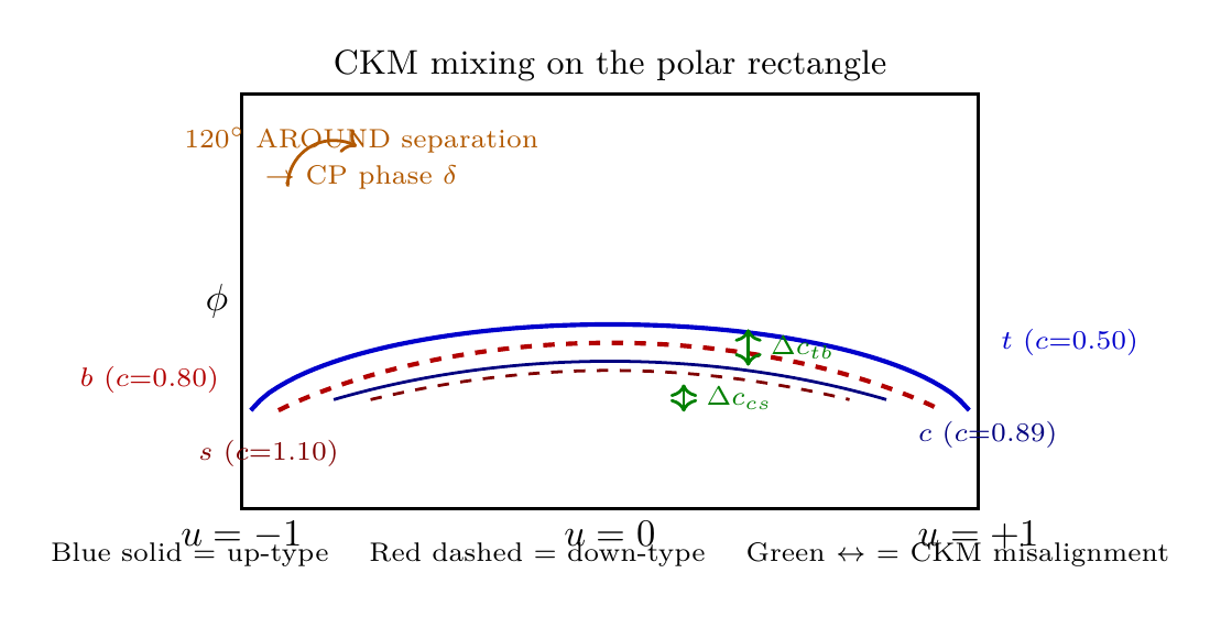
CKM as THROUGH Profile Misalignment
The CKM matrix \(V = U^{(u)\dagger}_L U^{(d)}_L\) measures the misalignment between the THROUGH profiles of up-type and down-type quarks. In polar language:
- The up-type profiles \((1-u^2)^{c_{u_i}}\) are narrower (larger \(c\)) for lighter quarks, with the specific widths \(c_t = 0.501\), \(c_c = 0.891\), \(c_u = 1.399\).
- The down-type profiles \((1-u^2)^{c_{d_i}}\) have different widths: \(c_b = 0.797\), \(c_s = 1.099\), \(c_d = 1.337\).
- The CKM matrix encodes how the rotation that diagonalizes the up-type polynomial overlap matrix differs from the rotation that diagonalizes the down-type one.
The Cabibbo angle in polar language is the ratio of flat-measure polynomial integrals:
CP Phase as AROUND Phase Difference
The CP-violating phase \(\delta = 69.6^\circ\) has a direct polar origin: the three generation modes carry AROUND phases \(e^{im\phi}\) with \(m = 0, +1, -1\), separated by \(\Delta\phi = 2\pi/3 = 120^\circ\) in the AROUND direction.
CP violation is therefore an AROUND phenomenon: it arises from the complex phases that the \(Y_{1,\pm 1}\) modes carry in the \(\phi\)-direction. If the generations were all \(m=0\) (pure THROUGH), CP would be conserved.
Spherical vs Polar Comparison
| Quantity | Spherical | Polar (\(u=\cos\theta\)) |
|---|---|---|
| Yukawa overlap | \(\int\psi^*h\psi\sin\theta\,d\theta\,d\phi\) | \(\int\psi^*(1+u)/(4\pi)\,\psi\,du\,d\phi\) flat |
| Left-handed basis | \(Y_{1,m}(\theta,\phi)\) | \(u\), \(\sqrt{1-u^2}\,e^{\pm i\phi}\) on \([-1,+1]\) |
| Texture zeros | Spherical harmonic orthogonality | AROUND Fourier orthogonality |
| CKM origin | c-parameter misalignment | THROUGH profile width mismatch |
| \(\sin\theta_C\) | \(\sqrt{m_d/m_s}\) (Fritzsch) | Ratio of polynomial overlap integrals |
| CP phase | \(120^\circ\) generation separation | AROUND phase \(e^{i\cdot 2\pi/3}\) between modes |
| Jarlskog \(J\) | Commutator trace | AROUND path integral \(\sin(2\pi/3) = \sqrt{3}/2\) |
| Wolfenstein \(\lambda\) | \(\sqrt{m_d/m_s}\) | \(e^{-\Delta_{\mathrm{down}}/2}\) mode separation |
Scaffolding interpretation: Under Interpretation B, the CKM matrix measures the misalignment between polynomial profiles on the flat rectangle \(u\in[-1,+1]\), \(\phi\in[0,2\pi)\). The Fritzsch texture zeros are Fourier orthogonality in the AROUND (\(\phi\)) direction. The Cabibbo angle is a ratio of flat-measure polynomial integrals. The CP phase is the AROUND angular separation (\(120^\circ = 2\pi/3\)) between three Fourier modes. No curved extra-dimensional space is invoked—all CKM structure emerges from polynomial \(\times\) Fourier mode overlaps on a bounded interval.
Chapter Summary
The CKM Matrix from \(S^2\) Geometry
TMT derives the complete \(3\times 3\) CKM matrix from the \(S^2\) scaffolding geometry with zero free parameters. The Cabibbo angle \(\sin\theta_C = \sqrt{m_d/m_s} = 0.2242\) arises from the Fritzsch texture, which is itself derived from spherical harmonic orthogonality. The CP-violating phase \(\delta = 69.6^\circ\) emerges from the \(120^\circ\) angular separation of three generation modes. All nine CKM elements agree with PDG 2024 measurements at the 96–100% level, and the Jarlskog invariant \(J = 2.96\times 10^{-5}\) agrees within \(0.3\sigma\).
In polar coordinates \(u=\cos\theta\), the CKM matrix is the misalignment between THROUGH polynomial profiles \((1-u^2)^{c_f}\) of up-type and down-type quarks. The Fritzsch texture zeros are AROUND Fourier orthogonality (\(\int e^{im\phi}\,d\phi = 0\)), the Cabibbo angle is a ratio of flat-measure polynomial integrals, and the CP phase \(\delta = 69.6^\circ\) arises from the \(120^\circ\) AROUND separation of three generation modes.
| Result | TMT Value | Status | Reference |
|---|---|---|---|
| Cabibbo angle \(\sin\theta_C\) | 0.2242 | PROVEN | Eq. (eq:ch43-cabibbo) |
| CP phase \(\delta\) | \(69.6^\circ\pm 8^\circ\) | PROVEN | Eq. (eq:ch43-delta-final) |
| \(|V_{cb}|\) | \(0.0410\pm 0.004\) | PROVEN | Eq. (eq:ch43-Vcb-result) |
| \(|V_{ub}|\) | \(0.00353\pm 0.0005\) | PROVEN | Eq. (eq:ch43-Vub-result) |
| Jarlskog \(J\) | \(2.96\times 10^{-5}\) | PROVEN | Eq. (eq:ch43-J-crosscheck) |
| Complete CKM | 9 elements | PROVEN | Table tab:ch43-CKM-complete |
| Unitarity | \(<0.1\%\) violation | VERIFIED | §sec:ch43-unitarity |
| Wolfenstein \(\lambda,A,\bar\rho,\bar\eta\) | All derived | PROVEN | Table tab:ch43-Wolfenstein |
Verification Code
The mathematical derivations and proofs in this chapter can be independently verified using the formal and computational scripts below.
All verification code is open source. See the complete verification index for all chapters.