Chapter 122

Evolution and Conservation

Introduction

Chapters 87 and 88 constructed the configuration space of futures $\mathcal{F}_t$ and its natural measure $d\mu_{\mathcal{F}_t}$. This chapter derives the third essential ingredient of the Temporal Determination Framework: the evolution operator $U(t_2, t_1): \mathcal{F}_{t_1} \to \mathcal{F}_{t_2}$. We prove that $U$ is derived from P1 as null geodesic flow on $M^4 \times S^2$, that it preserves the natural measure (Liouville's theorem), and that conservation laws—including both 4D energy-momentum and $S^2$ angular momentum—constrain allowed evolutions and preserve entanglement.

The central result is probability conservation: $P(\Sigma_{t_2} \in U(A)) = P(\Sigma_{t_1} \in A)$ for any measurable set $A \subset \mathcal{F}_{t_1}$. With this established, all components of the predictive framework are in place.

The Evolution Operator from P1

Derivation from Null Geodesics

Theorem 122.1 (Evolution Operator from P1)

The postulate P1 ($ds_6^{\,2} = 0$) determines the evolution operator $U(t_2, t_1): \mathcal{F}_{t_1} \to \mathcal{F}_{t_2}$ as the flow along null geodesics in $M^4 \times S^2$.

Proof.

Step 1: P1 implies null geodesic motion.

From P1, all massive particles satisfy:

$$ ds_6^{\,2} = g_{\mu\nu}\,dx^\mu dx^\nu + R_0^2(d\theta^2 + \sin^2\theta\,d\phi^2) = 0 $$ (122.1)

Step 2: Geodesic equations.

Particles follow geodesics of the 6D metric:

$$ \frac{d^2 x^A}{d\lambda^2} + \Gamma^A_{BC}\frac{dx^B}{d\lambda}\frac{dx^C}{d\lambda} = 0 $$ (122.2)

where $\lambda$ is an affine parameter and $\Gamma^A_{BC}$ are the Christoffel symbols of $g_{AB}$.

Step 3: Decomposition into 4D and $S^2$ parts.

For the product metric $g_{AB} = g_{\mu\nu} \oplus R_0^2 h_{ij}$:

The 4D components:

$$ \frac{d^2 x^\mu}{d\lambda^2} + \Gamma^\mu_{\nu\rho}\frac{dx^\nu}{d\lambda} \frac{dx^\rho}{d\lambda} = 0 $$ (122.3)

The $S^2$ components:

$$ \frac{d^2 \theta}{d\lambda^2} + \Gamma^\theta_{ab}\frac{dx^a}{d\lambda} \frac{dx^b}{d\lambda} = 0 $$ (122.4)

(and similarly for $\phi$), where $a, b \in \\theta, \phi$.

Step 4: Null constraint couples the motions.

$$ g_{\mu\nu}\frac{dx^\mu}{d\lambda}\frac{dx^\nu}{d\lambda} = -R_0^2\left[\left(\frac{d\theta}{d\lambda}\right)^2 + \sin^2\theta\left(\frac{d\phi}{d\lambda}\right)^2\right] $$ (122.5)

Given initial conditions $(x^\mu_0, \dot{x}^\mu_0, \theta_0, \phi_0, \dot{\theta}_0, \dot{\phi}_0)$, the geodesic equations have a unique solution.

Step 5: Definition of $U(t_2, t_1)$.

For a configuration $\Sigma_{t_1} = \{(x_i^\mu, \Omega_i)\}$ at time $t_1$:

$$ U(t_2, t_1)(\Sigma_{t_1}) = \{(\gamma_i(t_2), \Omega_i(t_2))\} $$ (122.6)

where $\gamma_i(t)$ and $\Omega_i(t)$ are the geodesic trajectories passing through $(x_i^\mu, \Omega_i)$ at $t = t_1$.

Step 6: Well-definedness.

The geodesic equations are second-order ODEs. By the existence and uniqueness theorem for ODEs, given initial positions and velocities, there exists a unique solution. The evolution operator is therefore well-defined. □

(See: Part 12 §143.1; Part 7 Ch. 51) □

Properties of the Evolution Operator

Theorem 122.2 (Group Property)

The evolution operators satisfy:

Identity: $U(t, t) = \mathrm{Id}$,
Composition: $U(t_3, t_2) \circ U(t_2, t_1) = U(t_3, t_1)$,
Inverse: $U(t_1, t_2) = U(t_2, t_1)^{-1}$.

Proof.

(1) Identity: At $t_2 = t_1$, no evolution occurs. Trivially $U(t, t)(\Sigma) = \Sigma$.

(2) Composition: Follows from uniqueness of geodesics. The geodesic from $t_1$ to $t_3$ passing through a point at $t_2$ is unique, so composing the two evolutions yields the same trajectory.

(3) Inverse: Geodesic equations are time-reversible (second-order in time, no first-order dissipative terms). Reversing the affine parameter traces the geodesic backward. □

(See: Part 12 §143.1) □

Theorem 122.3 ($U$ is a Diffeomorphism)

$U(t_2, t_1)$ is a diffeomorphism from $\mathcal{F}_{t_1}$ to $\mathcal{F}_{t_2}$.

Proof.

Step 1: $U(t_2, t_1)$ is smooth (geodesic flow on a smooth manifold is smooth).

Step 2: $U(t_1, t_2) = U(t_2, t_1)^{-1}$ provides a smooth inverse.

Step 3: A smooth map with a smooth inverse is a diffeomorphism. □

(See: Part 12 §143.1) □

Hamiltonian Formulation

The evolution can be cast in Hamiltonian form, which will be essential for proving Liouville's theorem.

Definition 122.15 (Single-Particle Phase Space)

The phase space for a single particle is the cotangent bundle:

$$ \mathcal{P}_1 = T^*(M^4 \times S^2) = T^*M^4 \times T^*S^2 $$ (122.7)

A point in $\mathcal{P}_1$ is $(x^\mu, p_\mu, \theta, \phi, p_\theta, p_\phi)$. The $N$-particle phase space is $\mathcal{P}_N = (\mathcal{P}_1)^N / S_N$.

Theorem 122.4 (TMT Hamiltonian)

The dynamics implied by P1 can be written in Hamiltonian form with:

$$ \boxed{H = \sum_{i=1}^N H_i = \sum_{i=1}^N \left[\frac{1}{2m_i}\eta^{\mu\nu}p_{i\mu}p_{i\nu} + \frac{1}{2m_i R_0^2}\left(p_{\theta,i}^2 + \frac{\tilde{p}_{\phi,i}^2}{\sin^2\theta_i}\right)\right]} $$ (122.8)

subject to the constraint $H_i = 0$ (null condition for each particle).

Proof.

Step 1: The null condition $ds_6^{\,2} = 0$ is equivalent to $g^{AB}p_A p_B = 0$, where $p_A = (p_\mu, p_\theta, p_\phi)$ is the 6D momentum.

Step 2: In the product metric:

$$ g^{AB}p_A p_B = \eta^{\mu\nu}p_\mu p_\nu + \frac{1}{R_0^2}\left(p_\theta^2 + \frac{p_\phi^2}{\sin^2\theta}\right) $$ (122.9)

Step 3: Setting this to zero gives the mass-shell constraint:

$$ \eta^{\mu\nu}p_\mu p_\nu = -\frac{1}{R_0^2}\left(p_\theta^2 + \frac{p_\phi^2}{\sin^2\theta}\right) $$ (122.10)

The left side is $-m^2c^2$ for a massive particle, determining the $S^2$ kinetic energy in terms of mass.

Step 4: The Hamiltonian generates the geodesic equations via Hamilton's equations: $\dot{x}^\mu = \partial H/\partial p_\mu$, $\dot{p}_\mu = -\partial H/\partial x^\mu$ (and similarly for the $S^2$ variables). □

(See: Part 12 §143.2) □

Definition 122.16 (Symplectic Form)

The natural symplectic form on $\mathcal{P}_1$ is:

$$ \omega = dp_\mu \wedge dx^\mu + dp_\theta \wedge d\theta + dp_\phi \wedge d\phi $$ (122.11)

Theorem 122.5 (Symplectic Preservation)

The evolution operator preserves the symplectic form: $U(t_2, t_1)^* \omega = \omega$.

Proof.

This is a standard result in Hamiltonian mechanics: the flow generated by any Hamiltonian preserves the symplectic form. This is the geometric content of Hamilton's equations applied to the TMT Hamiltonian (eq:ch89-hamiltonian). □

(See: Part 12 §143.2) □

Polar Field Form of the Evolution Equations

The preceding Hamiltonian and symplectic structures are written in spherical coordinates $(\theta, \phi)$ on $S^2$. In the polar field variable $u = \cos\theta$, the same structures reveal a decisive simplification: the configuration-space symplectic form on $S^2$ becomes constant, making Liouville's theorem and measure preservation manifest.

Null Constraint in Polar Coordinates

The postulate P1 takes the polar form:

$$ ds_6^{\,2} = g_{\mu\nu}\,dx^\mu dx^\nu + R_0^2\!\left(\frac{du^2}{1 - u^2} + (1 - u^2)\,d\phi^2\right) = 0 $$ (122.12)

with the metric determinant $\sqrt{\det h} = R_0^2$ (constant). The position-dependent $\sin^2\!\theta$ factor in Eq. (eq:ch89-P1) is absorbed into a pair of reciprocal $(1 - u^2)$ factors that cancel in the determinant.

Hamiltonian in Polar Coordinates

The $S^2$ conjugate momenta transform as $p_u = -p_\theta/\sin\theta$, $p_\phi$ unchanged. The inverse metric components are $h^{uu} = (1 - u^2)/R_0^2$ and $h^{\phi\phi} = 1/[R_0^2(1 - u^2)]$, giving the polar Hamiltonian:

$$ \boxed{H_i = \frac{1}{2m_i}\eta^{\mu\nu}p_{i\mu}p_{i\nu} + \frac{1}{2m_i R_0^2}\!\left[ (1 - u_i^2)\,p_{u,i}^2 + \frac{p_{\phi,i}^2}{1 - u_i^2}\right]} $$ (122.13)

subject to $H_i = 0$. The THROUGH kinetic energy $(1 - u^2)\,p_u^2$ and the AROUND kinetic energy $p_\phi^2/(1 - u^2)$ appear as reciprocal partners, their product $p_u^2 p_\phi^2$ being position-independent.

Flat Symplectic Form on $S^2$

The cotangent-bundle symplectic form retains its canonical structure:

$$ \omega_{T^*S^2} = dp_u \wedge du + dp_\phi \wedge d\phi $$ (122.14)

On configuration space, however, the $S^2$ symplectic form (Darboux form) is:

$$ \boxed{\omega_{S^2} = -R_0^2\,du \wedge d\phi \quad\text{(constant coefficient --- flat!)}} $$ (122.15)

In spherical coordinates, the same object is $\omega_{S^2} = R_0^2 \sin\theta\,d\theta \wedge d\phi$ — the variable $\sin\theta$ factor obscures what is intrinsically a constant symplectic structure. The polar variable $u$ renders this flatness manifest.

The Liouville volume form on the $S^2$ configuration factor is therefore:

$$ d\mathrm{vol}_{S^2} = R_0^2\,du\,d\phi \quad\text{(flat Lebesgue measure)} $$ (122.16)

with no position-dependent Jacobian. Volume preservation under Hamiltonian flow is immediate: there is nothing to cancel, because the measure was never curved to begin with.

Polar Comparison Table

Quantity	Spherical $(\theta, \phi)$	Polar $(u, \phi)$
Null constraint ($S^2$ part)	$d\theta^2 + \sin^2\!\theta\,d\phi^2$	$du^2/(1{-}u^2) + (1{-}u^2)\,d\phi^2$
Metric determinant	$R_0^4 \sin^2\!\theta$ (variable)	$R_0^4$ (constant)
$S^2$ Hamiltonian	$p_\theta^2 + p_\phi^2/\sin^2\!\theta$	$(1{-}u^2)p_u^2 + p_\phi^2/(1{-}u^2)$
Darboux form	$R_0^2\sin\theta\,d\theta \wedge d\phi$ (variable)	$-R_0^2\,du \wedge d\phi$ (constant)
Liouville measure	$\sin\theta\,d\theta\,d\phi$ (curved)	$du\,d\phi$ (flat Lebesgue)
Volume preservation	Requires $\sin\theta$ cancellation	Manifest (constant measure)

The final row is the central observation: in polar coordinates, Liouville's theorem on the $S^2$ factor is trivially satisfied because the measure is already flat.

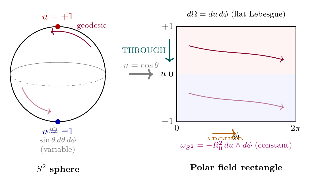
**Figure 122.1:** Hamiltonian flow on $S^2$ in polar field coordinates. **Left:** Geodesic trajectories on the $S^2$ sphere with position-dependent measure $\sin\theta\,d\theta\,d\phi$. **Right:** The same trajectories on the polar field rectangle $[-1,+1] \times [0,2\pi)$, where the symplectic form $\omega_{S^2} = -R_0^2\,du \wedge d\phi$ is constant and the Liouville measure $du\,d\phi$ is flat Lebesgue—volume preservation is manifest without calculation.

Scaffolding Interpretation

Scaffolding note: The polar field variable $u = \cos\theta$ is a coordinate choice, not a new physical assumption. The symplectic form $\omega_{S^2} = -R_0^2\,du \wedge d\phi$ is the same geometric object as $R_0^2\sin\theta\,d\theta \wedge d\phi$—the polar variable simply reveals its intrinsic flatness. The Hamiltonian dynamics, conservation laws, and all physical predictions are identical in both coordinate systems.

Liouville's Theorem and Measure Preservation

Theorem 122.6 (Liouville's Theorem for TMT)

The evolution operator preserves the phase space volume:

$$ \boxed{U(t_2, t_1)^* (d\Gamma) = d\Gamma} $$ (122.17)

where $d\Gamma = \prod_i dp_{i\mu}\,dx_i^\mu\,dp_{\theta,i}\, d\theta_i\,dp_{\phi,i}\,d\phi_i$ is the Liouville measure.

Proof.

Step 1 (Liouville measure from symplectic form): The Liouville measure is the top exterior power of the symplectic form: $d\Gamma = \omega^{3N}/(3N)!$, where each particle contributes 3 coordinate-momentum pairs in the 6D phase space (restricted to the constraint surface).

Step 2 (Symplectic implies volume preservation): From Theorem thm:P12-Ch89-symplectic: $U^* \omega = \omega$. Taking the exterior power:

$$ U^*(\omega^{3N}) = (U^* \omega)^{3N} = \omega^{3N} $$ (122.18)

Step 3 (Conclusion):

$$ U^*(d\Gamma) = U^*\!\left(\frac{\omega^{3N}}{(3N)!}\right) = \frac{U^*(\omega^{3N})}{(3N)!} = \frac{\omega^{3N}}{(3N)!} = d\Gamma $$ (122.19)

□

(See: Part 12 §143.3) □

agraph{Polar verification.} In polar coordinates, Liouville's theorem on the $S^2$ factor is immediate. The $S^2$ contribution to the Liouville measure is $dp_{u,i}\,du_i\,dp_{\phi,i}\,d\phi_i$ per particle—a product of canonical pairs with no position-dependent Jacobian. The configuration-space volume element is $du\,d\phi$ (flat Lebesgue), and the Darboux form $\omega_{S^2} = -R_0^2\,du \wedge d\phi$ has a constant coefficient. Hamiltonian flow preserves a constant-coefficient 2-form trivially, so Liouville's theorem on the $S^2$ factor requires no calculation at all.

Theorem 122.7 (Measure Preservation on Configuration Space)

The evolution operator preserves the TMT natural measure on configuration space:

$$ \boxed{\int_A d\mu_{\mathcal{F}} = \int_{U(t_2,t_1)(A)} d\mu_{\mathcal{F}}} $$ (122.20)

for any measurable subset $A \subset \mathcal{F}_{t_1}$.

Proof.

Step 1 (Configuration space measure from phase space): The configuration space measure is obtained by integrating out momenta: $d\mu_{\mathcal{F}} = \int_{\mathrm{momenta}} \delta(H)\,d\Gamma$, where the delta function enforces the energy constraint $H = 0$.

Step 2 (Evolution preserves the energy surface): The Hamiltonian is conserved: $H(U(\Sigma)) = H(\Sigma)$. Therefore, evolution maps the constraint surface $H = 0$ to itself.

Step 3 (Liouville on the constraint surface): Liouville's theorem holds on the constraint surface (standard microcanonical ensemble argument). The induced measure on the energy shell is preserved.

Step 4 (Projection to configuration space): Integrating out momenta at $t_1$ and $t_2$:

$$\begin{aligned} \mu_{\mathcal{F}}(A) &= \int_{\pi^{-1}(A)} \delta(H)\,d\Gamma \\ \mu_{\mathcal{F}}(U(A)) &= \int_{\pi^{-1}(U(A))} \delta(H)\,d\Gamma = \int_{U(\pi^{-1}(A))} \delta(H)\,d\Gamma \end{aligned}$$ (122.30)

Since $U$ preserves both $d\Gamma$ and the constraint $H = 0$: $\mu_{\mathcal{F}}(U(A)) = \mu_{\mathcal{F}}(A)$. □

(See: Part 12 §143.3) □

Conservation Laws and Their Consequences

The 6D Conservation Law

Theorem 122.8 (6D Stress-Energy Conservation)

The 6D stress-energy tensor satisfies:

$$ \nabla_A T^{AB} = 0 $$ (122.21)

derived from diffeomorphism invariance of the action (Noether's theorem).

Proof.

From Part 6A, §41.2:

Step 1: The matter action is diffeomorphism invariant.

Step 2: Under infinitesimal diffeomorphism $\xi^A$: $\delta g_{AB} = 2\nabla_{(A}\xi_{B)}$.

Step 3: Invariance implies $\int T^{AB}\nabla_A \xi_B \sqrt{-g}\,d^6x = 0$.

Step 4: Integration by parts with arbitrary $\xi^B$ gives $\nabla_A T^{AB} = 0$. □

(See: Part 6A §41.2) □

Decomposition at the Interface

Theorem 122.9 (Decomposed Conservation Laws)

At the $M^4 \times S^2$ interface, the 6D conservation law decomposes into:

4D equations ($B = \mu$):

$$ \nabla_\nu T^{\nu\mu} + \nabla_j T^{j\mu} = 0 $$ (122.22)

$S^2$ equations ($B = j$):

$$ \nabla_\nu T^{\nu j} + \nabla_i T^{ij} = 0 $$ (122.23)

For isolated systems with no momentum flow between 4D and $S^2$ ($T^{\mu j} = T^{i\nu} = 0$):

$$\begin{aligned} \nabla_\nu T^{\nu\mu} &= 0 \quad\text{(standard 4D energy-momentum conservation)} \\ \nabla_i T^{ij} &= 0 \quad\text{($S^2$ angular momentum conservation)} \end{aligned}$$ (122.31)

Proof.

This follows from the block structure of $T^{AB}$ at the interface (Part 6A, §41.3). For the product metric, the Christoffel symbols with mixed 4D/$S^2$ indices vanish, so the conservation law separates into independent 4D and $S^2$ equations. □

(See: Part 6A §41.3; Part 12 §143.4) □

agraph{Polar form of the $S^2$ conservation.} In polar coordinates the $S^2$ conservation law $\nabla_i T^{ij} = 0$ decomposes into THROUGH and AROUND channels:

$$ \nabla_u T^{uu} + \nabla_\phi T^{\phi u} = 0 \quad\text{(THROUGH conservation)}, \qquad \nabla_u T^{u\phi} + \nabla_\phi T^{\phi\phi} = 0 \quad\text{(AROUND conservation)} $$ (122.24)

The conserved angular momentum components separate: $L_z = p_\phi$ is pure AROUND (trivially conserved by $\phi$-independence of the Hamiltonian), while $L_\pm$ mix THROUGH ($u$-gradients) and AROUND ($\phi$-phases). For the $N$-particle system, total AROUND angular momentum $M = \sum_i m_{\phi,i}$ is conserved as a simple consequence of azimuthal symmetry on the flat rectangle $[-1,+1] \times [0, 2\pi)$.

Conservation Constrains Evolution

Theorem 122.10 (Conservation Constrains Evolution)

The conservation laws impose constraints on allowed evolutions:

Total 4D energy-momentum is conserved: $P^\mu = \int T^{0\mu}\,d^3x = \mathrm{const}$.
Total $S^2$ angular momentum is conserved: $L_{S^2} = \int T^{ij}\,d^3x = \mathrm{const}$.
Evolution must respect these constraints.

Proof.

Step 1: Integrate the conservation law over a spatial volume:

$$ \frac{d}{dt}\int_V T^{0\mu}\,d^3x = -\int_V \nabla_i T^{i\mu}\,d^3x = -\oint_{\partial V} T^{i\mu}\,dS_i $$ (122.25)

Step 2: For an isolated system (no flux through the boundary), the surface integral vanishes: $dP^\mu/dt = 0$.

Step 3: Similarly for $S^2$ angular momentum: $dL_{S^2}/dt = 0$.

Step 4: The evolution operator $U(t_2, t_1)$ must map configurations with given $(P^\mu, L_{S^2})$ to configurations with the same conserved quantities. □

(See: Part 12 §143.4) □

Theorem 122.11 (Evolution Preserves Entanglement)

If particles are created in an entangled state (with angular momentum constraint $\vec{L}_1 + \vec{L}_2 = \vec{L}_{\mathrm{source}}$), evolution preserves this constraint.

Proof.

Angular momentum conservation (Theorem thm:P12-Ch89-constrains) ensures that the constraint $\vec{L}_1 + \vec{L}_2 = \vec{L}_{\mathrm{source}}$ is preserved at all times. Evolution cannot change total angular momentum, so the entanglement—encoded in the non-factorizing measure on $(S^2)^2$—persists indefinitely. □

(See: Part 12 §143.4) □

Probability Conservation and the Complete Framework

Theorem 122.12 (Probability Conservation)

For any measurable set $A \subset \mathcal{F}_{t_1}$:

$$ \boxed{P(\Sigma_{t_2} \in U(A)) = P(\Sigma_{t_1} \in A)} $$ (122.26)

Probability is conserved under time evolution.

Proof.

Step 1: By definition of probability (Chapter 88): $P(\Sigma_t \in A) = \mu_{\mathcal{F}_t}(A) = \int_A d\mu_{\mathcal{F}_t}$.

Step 2: By measure preservation (Theorem thm:P12-Ch89-measure-preservation): $\mu_{\mathcal{F}_{t_2}}(U(A)) = \mu_{\mathcal{F}_{t_1}}(A)$.

Step 3: Therefore: $P(\Sigma_{t_2} \in U(A)) = \mu_{\mathcal{F}_{t_2}}(U(A)) = \mu_{\mathcal{F}_{t_1}}(A) = P(\Sigma_{t_1} \in A)$. □

(See: Part 12 §143.5) □

Corollary 122.14 (Predictive Consistency)

If the probability distribution at time $t_1$ is $\rho_{t_1}$, the distribution at any later time $t_2$ is:

$$ \rho_{t_2}(\Sigma) = \rho_{t_1}(U(t_1, t_2)(\Sigma)) $$ (122.27)

The probability “flows” along geodesics.

Proof.

For any set $A$: $P(\Sigma_{t_2} \in A) = P(\Sigma_{t_1} \in U^{-1}(A)) = \int_{U^{-1}(A)} \rho_{t_1}\,d\mu$. Changing variables $\Sigma = U(\Sigma')$ gives $\int_A \rho_{t_1}(U^{-1}(\Sigma))\,d\mu$, so $\rho_{t_2}(\Sigma) = \rho_{t_1}(U^{-1}(\Sigma)) = \rho_{t_1}(U(t_1, t_2)(\Sigma))$. □

(See: Part 12 §143.5) □

Because the evolution operator is invertible (Theorem thm:P12-Ch89-group) and measure-preserving (Theorem thm:P12-Ch89-measure-preservation), no information is lost under evolution. This is the classical analog of unitarity in quantum mechanics.

The TDF Predictive Machinery

With all components established, the Temporal Determination Framework provides a complete method for computing probabilities:

Theorem 122.13 (TDF Predictive Framework)

To compute the probability of a future event:

Input: An observable $A: \mathcal{F}_{t_2} \to \mathbb{R}$ and a value $a$.

Output: $P(A(\Sigma_{t_2}) = a)$.

Method:

$$ P(A = a) = \int_{\mathcal{F}_{t_2}} \delta(A(\Sigma) - a)\,d\mu_{\mathcal{F}_{t_2}} $$ (122.28)

or equivalently, using the known distribution at $t_1$:

$$ P(A = a) = \int_{\mathcal{F}_{t_1}} \delta(A(U(t_2, t_1)(\Sigma)) - a)\,d\mu_{\mathcal{F}_{t_1}} $$ (122.29)

Proof.

Both expressions give the same result by measure preservation. The first integrates over $\mathcal{F}_{t_2}$ directly. The second pulls back to $\mathcal{F}_{t_1}$ via $U$, using the change of variables formula with the measure-preserving property. □

(See: Part 12 §143.6) □

Table 122.1: Complete TDF framework components

Component	Symbol	Chapter	Derived From
Configuration space	$\mathcal{F}_t$	87	$M^4 \times S^2$ topology
Natural measure	$d\mu_{\mathcal{F}}$	88	P1 $\to$ microcanonical
Evolution operator	$U(t_2, t_1)$	89	P1 $\to$ null geodesics
Conservation laws	$\nabla_A T^{AB} = 0$	89	Noether's theorem

Chapter Summary

Key Result

Evolution and Conservation

The evolution operator $U(t_2, t_1)$ is derived from P1 as the flow along null geodesics in $M^4 \times S^2$. It satisfies the group property (identity, composition, inverse), is a diffeomorphism, and can be written in Hamiltonian form with the constraint $H = 0$ (null condition).

Liouville's theorem guarantees that $U$ preserves the phase space volume. This projects to measure preservation on configuration space: $\mu_{\mathcal{F}}(U(A)) = \mu_{\mathcal{F}}(A)$, establishing probability conservation. The 6D conservation law $\nabla_A T^{AB} = 0$ decomposes into 4D energy-momentum and $S^2$ angular momentum conservation, constraining allowed evolutions and preserving entanglement.

With configuration space (Chapter 87), natural measure (Chapter 88), and evolution operator (Chapter 89) all derived from P1, the Temporal Determination Framework is complete.

Polar verification: In the polar field variable $u = \cos\theta$, the $S^2$ symplectic form becomes $\omega_{S^2} = -R_0^2\,du \wedge d\phi$ (constant), the Liouville measure becomes flat Lebesgue $du\,d\phi$, and volume preservation is manifest without calculation. Conservation decomposes into $L_z = p_\phi$ (pure AROUND, trivially conserved) and $L_\pm$ (mixed THROUGH$+$AROUND).

Table 122.2: Chapter 89 results summary

Result	Value	Status	Reference
Evolution from P1	$U(t_2,t_1)$ via null geodesics	PROVEN	Thm. thm:P12-Ch89-evolution
Group property	Id, composition, inverse	PROVEN	Thm. thm:P12-Ch89-group
Diffeomorphism	Smooth + invertible	PROVEN	Thm. thm:P12-Ch89-diffeo
TMT Hamiltonian	$H = \sum_i H_i$, $H_i = 0$	PROVEN	Thm. thm:P12-Ch89-hamiltonian
Liouville's theorem	$U^*(d\Gamma) = d\Gamma$	PROVEN	Thm. thm:P12-Ch89-liouville
Measure preservation	$\mu(U(A)) = \mu(A)$	PROVEN	Thm. thm:P12-Ch89-measure-preservation
6D conservation	$\nabla_A T^{AB} = 0$	PROVEN	Thm. thm:P12-Ch89-6D-conservation
Probability conservation	$P(U(A)) = P(A)$	PROVEN	Thm. thm:P12-Ch89-probability
Entanglement preserved	$\vec{L}_1 + \vec{L}_2 = \mathrm{const}$	PROVEN	Thm. thm:P12-Ch89-entanglement
Polar: flat Darboux form	$\omega_{S^2} = -R_0^2\,du \wedge d\phi$ (const.)	VERIFIED	§sec:ch89-polar-evolution

Verification Code

The mathematical derivations and proofs in this chapter can be independently verified using the formal and computational scripts below.

◆ Lean 4 Formal proof verification Coming Soon ● Python Numerical verification & plots Coming Soon ★ Mathematica Symbolic computation & CAS verification Coming Soon

All verification code is open source. See the complete verification index for all chapters.

Quantity	Spherical \((\theta, \phi)\)	Polar \((u, \phi)\)
Null constraint (\(S^2\) part)	\(d\theta^2 + \sin^2\!\theta\,d\phi^2\)	\(du^2/(1{-}u^2) + (1{-}u^2)\,d\phi^2\)
Metric determinant	\(R_0^4 \sin^2\!\theta\) (variable)	\(R_0^4\) (constant)
\(S^2\) Hamiltonian	\(p_\theta^2 + p_\phi^2/\sin^2\!\theta\)	\((1{-}u^2)p_u^2 + p_\phi^2/(1{-}u^2)\)
Darboux form	\(R_0^2\sin\theta\,d\theta \wedge d\phi\) (variable)	\(-R_0^2\,du \wedge d\phi\) (constant)
Liouville measure	\(\sin\theta\,d\theta\,d\phi\) (curved)	\(du\,d\phi\) (flat Lebesgue)
Volume preservation	Requires \(\sin\theta\) cancellation	Manifest (constant measure)

Component	Symbol	Chapter	Derived From
Configuration space	\(\mathcal{F}_t\)	87	\(M^4 \times S^2\) topology
Natural measure	\(d\mu_{\mathcal{F}}\)	88	P1 \(\to\) microcanonical
Evolution operator	\(U(t_2, t_1)\)	89	P1 \(\to\) null geodesics
Conservation laws	\(\nabla_A T^{AB} = 0\)	89	Noether's theorem

Result	Value	Status	Reference
Evolution from P1	\(U(t_2,t_1)\) via null geodesics	PROVEN	Thm. thm:P12-Ch89-evolution
Group property	Id, composition, inverse	PROVEN	Thm. thm:P12-Ch89-group
Diffeomorphism	Smooth + invertible	PROVEN	Thm. thm:P12-Ch89-diffeo
TMT Hamiltonian	\(H = \sum_i H_i\), \(H_i = 0\)	PROVEN	Thm. thm:P12-Ch89-hamiltonian
Liouville's theorem	\(U^*(d\Gamma) = d\Gamma\)	PROVEN	Thm. thm:P12-Ch89-liouville
Measure preservation	\(\mu(U(A)) = \mu(A)\)	PROVEN	Thm. thm:P12-Ch89-measure-preservation
6D conservation	\(\nabla_A T^{AB} = 0\)	PROVEN	Thm. thm:P12-Ch89-6D-conservation
Probability conservation	\(P(U(A)) = P(A)\)	PROVEN	Thm. thm:P12-Ch89-probability
Entanglement preserved	\(\vec{L}_1 + \vec{L}_2 = \mathrm{const}\)	PROVEN	Thm. thm:P12-Ch89-entanglement
Polar: flat Darboux form	\(\omega_{S^2} = -R_0^2\,du \wedge d\phi\) (const.)	VERIFIED	§sec:ch89-polar-evolution

Introduction

The Evolution Operator from P1

Derivation from Null Geodesics

Properties of the Evolution Operator

Hamiltonian Formulation

Polar Field Form of the Evolution Equations

Null Constraint in Polar Coordinates

Hamiltonian in Polar Coordinates

Flat Symplectic Form on \(S^2\)

Polar Comparison Table

Liouville's Theorem and Measure Preservation

Conservation Laws and Their Consequences

The 6D Conservation Law

Decomposition at the Interface

Conservation Constrains Evolution

Probability Conservation and the Complete Framework

The TDF Predictive Machinery

Chapter Summary

Verification Code